Functional examples

Below the functional solution to some common geodesic problems are given. In the first example the object-oriented solution is also given. The object-oriented solutions to the remaining problems can be found here.

Example 1: “A and B to delta”

Given two positions, A and B as latitudes, longitudes and depths relative to Earth, E.

Find the exact vector between the two positions, given in meters north, east, and down, and find the direction (azimuth) to B, relative to north. Assume WGS-84 ellipsoid. The given depths are from the ellipsoid surface. Use position A to define north, east, and down directions. (Due to the curvature of Earth and different directions to the North Pole, the north, east, and down directions will change (relative to Earth) for different places. A must be outside the poles for the north and east directions to be defined.)

Solution:

>>> import numpy as np
>>> import nvector as nv
>>> from nvector import rad, deg

>>> lat_EA, lon_EA, z_EA = rad(1), rad(2), 3
>>> lat_EB, lon_EB, z_EB = rad(4), rad(5), 6

Step1: Convert to n-vectors:

>>> n_EA_E = nv.lat_lon2n_E(lat_EA, lon_EA)
>>> n_EB_E = nv.lat_lon2n_E(lat_EB, lon_EB)

Step2: Find p_AB_E (delta decomposed in E).WGS-84 ellipsoid is default:

>>> p_AB_E = nv.n_EA_E_and_n_EB_E2p_AB_E(n_EA_E, n_EB_E, z_EA, z_EB)

Step3: Find R_EN for position A:

>>> R_EN = nv.n_E2R_EN(n_EA_E)

Step4: Find p_AB_N (delta decomposed in N).

>>> p_AB_N = np.dot(R_EN.T, p_AB_E).ravel()
>>> valtxt = '{0:8.2f}, {1:8.2f}, {2:8.2f}'.format(*p_AB_N)
>>> 'Ex1: delta north, east, down = {}'.format(valtxt)
'Ex1: delta north, east, down = 331730.23, 332997.87, 17404.27'

Step5: Also find the direction (azimuth) to B, relative to north:

>>> azimuth = np.arctan2(p_AB_N[1], p_AB_N[0])
>>> 'azimuth = {0:4.2f} deg'.format(deg(azimuth))
'azimuth = 45.11 deg'

OO-Solution:

>>> import numpy as np
>>> import nvector as nv
>>> wgs84 = nv.FrameE(name='WGS84')
>>> pointA = wgs84.GeoPoint(latitude=1, longitude=2, z=3, degrees=True)
>>> pointB = wgs84.GeoPoint(latitude=4, longitude=5, z=6, degrees=True)

Step1: Find p_AB_N (delta decomposed in N).

>>> p_AB_N = pointA.delta_to(pointB)
>>> x, y, z = p_AB_N.pvector.ravel()
>>> valtxt = '{0:8.2f}, {1:8.2f}, {2:8.2f}'.format(x, y, z)
>>> 'Ex1: delta north, east, down = {}'.format(valtxt)
'Ex1: delta north, east, down = 331730.23, 332997.87, 17404.27'

Step2: Also find the direction (azimuth) to B, relative to north:

>>> azimuth = p_AB_N.azimuth_deg[0]
>>> 'azimuth = {0:4.2f} deg'.format(azimuth)
'azimuth = 45.11 deg'

See also

Example 1 at www.navlab.net

Example 2: “B and delta to C”

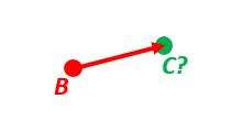
A radar or sonar attached to a vehicle B (Body coordinate frame) measures the distance and direction to an object C. We assume that the distance and two angles (typically bearing and elevation relative to B) are already combined to the vector p_BC_B (i.e. the vector from B to C, decomposed in B). The position of B is given as n_EB_E and z_EB, and the orientation (attitude) of B is given as R_NB (this rotation matrix can be found from roll/pitch/yaw by using zyx2R).

Find the exact position of object C as n-vector and depth ( n_EC_E and z_EC ), assuming Earth ellipsoid with semi-major axis a and flattening f. For WGS-72, use a = 6 378 135 m and f = 1/298.26.

Solution:

>>> import numpy as np
>>> import nvector as nv
>>> from nvector import rad, deg

A custom reference ellipsoid is given (replacing WGS-84):

>>> wgs72 = dict(a=6378135, f=1.0/298.26)

Step 1 Position and orientation of B is 400m above E:

>>> n_EB_E = nv.unit([[1], [2], [3]])  # unit to get unit length of vector
>>> z_EB = -400
>>> yaw, pitch, roll = rad(10), rad(20), rad(30)
>>> R_NB = nv.zyx2R(yaw, pitch, roll)

Step 2: Delta BC decomposed in B

>>> p_BC_B = np.r_[3000, 2000, 100].reshape((-1, 1))

Step 3: Find R_EN:

>>> R_EN = nv.n_E2R_EN(n_EB_E)

Step 4: Find R_EB, from R_EN and R_NB:

>>> R_EB = np.dot(R_EN, R_NB)  # Note: closest frames cancel

Step 5: Decompose the delta BC vector in E:

>>> p_BC_E = np.dot(R_EB, p_BC_B)

Step 6: Find the position of C, using the functions that goes from one

>>> n_EC_E, z_EC = nv.n_EA_E_and_p_AB_E2n_EB_E(n_EB_E, p_BC_E, z_EB, **wgs72)

>>> lat_EC, lon_EC = nv.n_E2lat_lon(n_EC_E)
>>> lat, lon, z = deg(lat_EC), deg(lon_EC), z_EC
>>> msg = 'Ex2: PosC: lat, lon = {:4.2f}, {:4.2f} deg,  height = {:4.2f} m'
>>> msg.format(lat[0], lon[0], -z[0])
'Ex2: PosC: lat, lon = 53.33, 63.47 deg,  height = 406.01 m'

See also

Example 2 at www.navlab.net

Example 3: “ECEF-vector to geodetic latitude”

Position B is given as an “ECEF-vector” p_EB_E (i.e. a vector from E, the center of the Earth, to B, decomposed in E). Find the geodetic latitude, longitude and height (latEB, lonEB and hEB), assuming WGS-84 ellipsoid.

Solution:

>>> import numpy as np
>>> import nvector as nv
>>> from nvector import deg
>>> wgs84 = dict(a=6378137.0, f=1.0/298.257223563)
>>> p_EB_E = 6371e3 * np.vstack((0.9, -1, 1.1))  # m

>>> n_EB_E, z_EB = nv.p_EB_E2n_EB_E(p_EB_E, **wgs84)

>>> lat_EB, lon_EB = nv.n_E2lat_lon(n_EB_E)
>>> h = -z_EB
>>> lat, lon = deg(lat_EB), deg(lon_EB)

>>> msg = 'Ex3: Pos B: lat, lon = {:4.2f}, {:4.2f} deg, height = {:9.2f} m'
>>> msg.format(lat[0], lon[0], h[0])
'Ex3: Pos B: lat, lon = 39.38, -48.01 deg, height = 4702059.83 m'

See also

Example 3 at www.navlab.net

Example 4: “Geodetic latitude to ECEF-vector”

Geodetic latitude, longitude and height are given for position B as latEB, lonEB and hEB, find the ECEF-vector for this position, p_EB_E.

Solution:

>>> import nvector as nv
>>> from nvector import rad
>>> wgs84 = dict(a=6378137.0, f=1.0/298.257223563)
>>> lat_EB, lon_EB = rad(1), rad(2)
>>> h_EB = 3
>>> n_EB_E = nv.lat_lon2n_E(lat_EB, lon_EB)
>>> p_EB_E = nv.n_EB_E2p_EB_E(n_EB_E, -h_EB, **wgs84)

>>> 'Ex4: p_EB_E = {} m'.format(p_EB_E.ravel().tolist())
'Ex4: p_EB_E = [6373290.277218279, 222560.20067473652, 110568.82718178593] m'

See also

Example 4 at www.navlab.net

Example 5: “Surface distance”

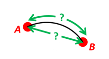
Find the surface distance sAB (i.e. great circle distance) between two positions A and B. The heights of A and B are ignored, i.e. if they don’t have zero height, we seek the distance between the points that are at the surface of the Earth, directly above/below A and B. The Euclidean distance (chord length) dAB should also be found. Use Earth radius 6371e3 m. Compare the results with exact calculations for the WGS-84 ellipsoid.

Solution for a sphere:

>>> import numpy as np
>>> import nvector as nv
>>> from nvector import rad

>>> n_EA_E = nv.lat_lon2n_E(rad(88), rad(0))
>>> n_EB_E = nv.lat_lon2n_E(rad(89), rad(-170))

>>> r_Earth = 6371e3  # m, mean Earth radius
>>> s_AB = nv.great_circle_distance(n_EA_E, n_EB_E, radius=r_Earth)[0]
>>> d_AB = nv.euclidean_distance(n_EA_E, n_EB_E, radius=r_Earth)[0]

>>> msg = 'Ex5: Great circle and Euclidean distance = {}'
>>> msg = msg.format('{:5.2f} km, {:5.2f} km')
>>> msg.format(s_AB / 1000, d_AB / 1000)
'Ex5: Great circle and Euclidean distance = 332.46 km, 332.42 km'

Exact solution for the WGS84 ellipsoid:

>>> wgs84 = nv.FrameE(name='WGS84')
>>> point1 = wgs84.GeoPoint(latitude=88, longitude=0, degrees=True)
>>> point2 = wgs84.GeoPoint(latitude=89, longitude=-170, degrees=True)
>>> s_12, _azi1, _azi2 = point1.distance_and_azimuth(point2)

>>> p_12_E = point2.to_ecef_vector() - point1.to_ecef_vector()
>>> d_12 = p_12_E.length[0]
>>> msg = 'Ellipsoidal and Euclidean distance = {:5.2f} km, {:5.2f} km'
>>> msg.format(s_12 / 1000, d_12 / 1000)
'Ellipsoidal and Euclidean distance = 333.95 km, 333.91 km'

See also

Example 5 at www.navlab.net

Example 6 “Interpolated position”

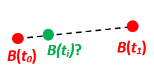
Given the position of B at time t0 and t1, n_EB_E(t0) and n_EB_E(t1).

Find an interpolated position at time ti, n_EB_E(ti). All positions are given as n-vectors.

Solution:

>>> import nvector as nv
>>> from nvector import rad, deg
>>> n_EB_E_t0 = nv.lat_lon2n_E(rad(89), rad(0))
>>> n_EB_E_t1 = nv.lat_lon2n_E(rad(89), rad(180))

>>> t0 = 10.
>>> t1 = 20.
>>> ti = 16.  # time of interpolation
>>> ti_n = (ti - t0) / (t1 - t0) # normalized time of interpolation

>>> n_EB_E_ti = nv.unit(n_EB_E_t0 + ti_n * (n_EB_E_t1 - n_EB_E_t0))
>>> lat_EB_ti, lon_EB_ti = nv.n_E2lat_lon(n_EB_E_ti)

>>> lat_ti, lon_ti = deg(lat_EB_ti), deg(lon_EB_ti)
>>> msg = 'Ex6, Interpolated position: lat, lon = {:2.1f} deg, {:2.1f} deg'
>>> msg.format(lat_ti[0], lon_ti[0])
'Ex6, Interpolated position: lat, lon = 89.8 deg, 180.0 deg'

See also

Example 6 at www.navlab.net

Example 7: “Mean position”

Three positions A, B, and C are given as n-vectors n_EA_E, n_EB_E, and n_EC_E. Find the mean position, M, given as n_EM_E. Note that the calculation is independent of the depths of the positions.

Solution:

>>> import numpy as np
>>> import nvector as nv
>>> from nvector import rad, deg

>>> n_EA_E = nv.lat_lon2n_E(rad(90), rad(0))
>>> n_EB_E = nv.lat_lon2n_E(rad(60), rad(10))
>>> n_EC_E = nv.lat_lon2n_E(rad(50), rad(-20))

>>> n_EM_E = nv.unit(n_EA_E + n_EB_E + n_EC_E)

or

>>> n_EM_E = nv.mean_horizontal_position(np.hstack((n_EA_E, n_EB_E, n_EC_E)))

>>> lat, lon = nv.n_E2lat_lon(n_EM_E)
>>> lat, lon = deg(lat), deg(lon)
>>> msg = 'Ex7: Pos M: lat, lon = {:4.2f}, {:4.2f} deg'
>>> msg.format(lat[0], lon[0])
'Ex7: Pos M: lat, lon = 67.24, -6.92 deg'

See also

Example 7 at www.navlab.net

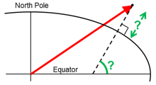
Example 8: “A and azimuth/distance to B”

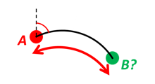
We have an initial position A, direction of travel given as an azimuth (bearing) relative to north (clockwise), and finally the distance to travel along a great circle given as sAB. Use Earth radius 6371e3 m to find the destination point B.

In geodesy this is known as “The first geodetic problem” or “The direct geodetic problem” for a sphere, and we see that this is similar to Example 2, but now the delta is given as an azimuth and a great circle distance. (“The second/inverse geodetic problem” for a sphere is already solved in Examples 1 and 5.)

Solution:

>>> import nvector as nv
>>> from nvector import rad, deg
>>> lat, lon = rad(80), rad(-90)

>>> n_EA_E = nv.lat_lon2n_E(lat, lon)
>>> azimuth = rad(200)
>>> s_AB = 1000.0  # [m]
>>> r_earth = 6371e3  # [m], mean earth radius

>>> distance_rad = s_AB / r_earth
>>> n_EB_E = nv.n_EA_E_distance_and_azimuth2n_EB_E(n_EA_E, distance_rad,
...                                                azimuth)
>>> lat_EB, lon_EB = nv.n_E2lat_lon(n_EB_E)
>>> lat, lon = deg(lat_EB), deg(lon_EB)
>>> msg = 'Ex8, Destination: lat, lon = {:4.2f} deg, {:4.2f} deg'
>>> msg.format(lat[0], lon[0])
'Ex8, Destination: lat, lon = 79.99 deg, -90.02 deg'

See also

Example 8 at www.navlab.net

Example 9: “Intersection of two paths”

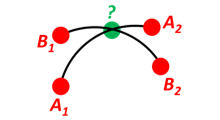
Define a path from two given positions (at the surface of a spherical Earth), as the great circle that goes through the two points.

Path A is given by A1 and A2, while path B is given by B1 and B2.

Find the position C where the two great circles intersect.

Solution:

>>> import numpy as np
>>> import nvector as nv
>>> from nvector import rad, deg

>>> n_EA1_E = nv.lat_lon2n_E(rad(10), rad(20))
>>> n_EA2_E = nv.lat_lon2n_E(rad(30), rad(40))
>>> n_EB1_E = nv.lat_lon2n_E(rad(50), rad(60))
>>> n_EB2_E = nv.lat_lon2n_E(rad(70), rad(80))

>>> n_EC_E = nv.unit(np.cross(np.cross(n_EA1_E, n_EA2_E, axis=0),
...                           np.cross(n_EB1_E, n_EB2_E, axis=0),
...                           axis=0))
>>> n_EC_E *= np.sign(np.dot(n_EC_E.T, n_EA1_E))

or alternatively

>>> path_a, path_b = (n_EA1_E, n_EA2_E), (n_EB1_E, n_EB2_E)
>>> n_EC_E = nv.intersect(path_a, path_b)

>>> lat_EC, lon_EC = nv.n_E2lat_lon(n_EC_E)

>>> lat, lon = deg(lat_EC), deg(lon_EC)
>>> msg = 'Ex9, Intersection: lat, lon = {:4.2f}, {:4.2f} deg'
>>> msg.format(lat[0], lon[0])
'Ex9, Intersection: lat, lon = 40.32, 55.90 deg'

>>> np.allclose(nv.on_great_circle_path(path_a, n_EC_E),
...             nv.on_great_circle_path(path_b, n_EC_E))
True
>>> np.allclose(nv.on_great_circle(path_a, n_EC_E), nv.on_great_circle(path_b, n_EC_E))
True

See also

Example 9 at www.navlab.net

Example 10: “Cross track distance”

Path A is given by the two positions A1 and A2 (similar to the previous example).

Find the cross track distance sxt between the path A (i.e. the great circle through A1 and A2) and the position B (i.e. the shortest distance at the surface, between the great circle and B).

Also find the Euclidean distance dxt between B and the plane defined by the great circle. Use Earth radius 6371e3.

Finally, find the intersection point on the great circle and determine if it is between position A1 and A2.

Solution:

>>> import numpy as np
>>> import nvector as nv
>>> n_EA1_E = nv.lat_lon2n_E(rad(0), rad(0))
>>> n_EA2_E = nv.lat_lon2n_E(rad(10), rad(0))
>>> n_EB_E = nv.lat_lon2n_E(rad(1), rad(0.1))
>>> path = (n_EA1_E, n_EA2_E)
>>> radius = 6371e3  # mean earth radius [m]
>>> s_xt = nv.cross_track_distance(path, n_EB_E, radius=radius)
>>> d_xt = nv.cross_track_distance(path, n_EB_E, method='euclidean',
...                                radius=radius)

>>> val_txt = '{:4.2f} km, {:4.2f} km'.format(s_xt[0]/1000, d_xt[0]/1000)
>>> 'Ex10: Cross track distance: s_xt, d_xt = {0}'.format(val_txt)
'Ex10: Cross track distance: s_xt, d_xt = 11.12 km, 11.12 km'

>>> n_EC_E = nv.closest_point_on_great_circle(path, n_EB_E)
>>> np.allclose(nv.on_great_circle_path(path, n_EC_E, radius), True)
True

Alternative solution 2:

>>> s_xt2 = nv.great_circle_distance(n_EB_E, n_EC_E, radius)
>>> d_xt2 = nv.euclidean_distance(n_EB_E, n_EC_E, radius)
>>> np.allclose(s_xt, s_xt2), np.allclose(d_xt, d_xt2)
(True, True)

Alternative solution 3:

>>> c_E = nv.great_circle_normal(n_EA1_E, n_EA2_E)
>>> sin_theta = -np.dot(c_E.T, n_EB_E).ravel()
>>> s_xt3 = np.arcsin(sin_theta) * radius
>>> d_xt3 = sin_theta * radius
>>> np.allclose(s_xt, s_xt3), np.allclose(d_xt, d_xt3)
(True, True)

See also

Example 10 at www.navlab.net