5.1. Object-oriented interface to geodesic functions

5.1.1. Classes in module

FrameB:

Body frame

FrameE:

Earth-fixed frame

FrameN:

North-East-Down frame

FrameL:

Local level, Wander azimuth frame

GeoPath:

Geographical path between two positions in Frame E

GeoPoint:

Geographical position(s) given as latitude(s), longitude(s), depth(s) in frame E.

ECEFvector:

Geographical position(s) given as cartesian position vector(s) in frame E

Nvector:

Geographical position(s) given as n-vector(s) and depth(s) in frame E

Pvector:

Geographical position(s) given as cartesian position vector(s) in a frame.

5.1.2. Functions in module

delta_E:

Returns cartesian delta vector from positions A to B decomposed in E.

delta_L:

Returns cartesian delta vector from positions A to B decomposed in L.

delta_N:

Returns cartesian delta vector from positions A to B decomposed in N.

class nvector.objects.ECEFvector(pvector: List[Any] | Tuple[Any, ...] | ndarray[tuple[Any, ...], dtype[Any]], frame: FrameE | None = None, scalar: bool | None = None)

Geographical position(s) given as cartesian position vector(s) in frame E

pvector

3 x n array cartesian position vector(s) [m] from E to B, decomposed in E.

Type:

ndarray

frame

Reference ellipsoid. The default ellipsoid model used is WGS84, but other ellipsoids/spheres might be specified.

Type:

FrameE

scalar

True if p-vector represents a scalar position, i.e. n = 1.

Type:

bool

Notes

The position of B (typically body) relative to E (typically Earth) is given into this function as p-vector, p_EB_E relative to the center of the frame.

Examples

Example 3: “ECEF-vector to geodetic latitude”

Position B is given as an “ECEF-vector” p_EB_E (i.e. a vector from E, the center of the Earth, to B, decomposed in E). Find the geodetic latitude, longitude and height (latEB, lonEB and hEB), assuming WGS-84 ellipsoid.

Solution:

>>> import numpy as np
>>> import nvector as nv
>>> wgs84 = nv.FrameE(name="WGS84")
>>> position_B = 6371e3 * np.vstack((0.9, -1, 1.1))  # m
>>> p_EB_E = wgs84.ECEFvector(position_B)

Step 1: Find geodetic latitude and depth from the p-vector:

>>> pointB = p_EB_E.to_geo_point()

>>> lat, lon, z = pointB.latlon_deg
>>> "Ex3: Pos B: lat, lon = {:4.4f}, {:4.4f} deg, height = {:9.3f} m".format(lat, lon, -z)
'Ex3: Pos B: lat, lon = 39.3787, -48.0128 deg, height = 4702059.834 m'

Example 4: “Geodetic latitude to ECEF-vector”

Geodetic latitude, longitude and height are given for position B as latEB, lonEB and hEB, find the ECEF-vector for this position, p_EB_E.

Solution:

>>> import nvector as nv
>>> wgs84 = nv.FrameE(name="WGS84")
>>> pointB = wgs84.GeoPointFromDegrees(latitude=1, longitude=2, z=-3)
>>> p_EB_E = pointB.to_ecef_vector()

>>> "Ex4: p_EB_E = {} m".format(p_EB_E.pvector.ravel().tolist())
'Ex4: p_EB_E = [6373290.277218279, 222560.20067473652, 110568.82718178593] m'

See also

GeoPoint, ECEFvector, Pvector

change_frame(frame: FrameB | FrameL | FrameN) → Pvector

Converts to Cartesian position vector in another frame

Parameters:

frame (FrameB, FrameN or FrameL) – Local frame M used to convert p_AB_E (position vector from A to B, decomposed in E) to a cartesian vector p_AB_M decomposed in M.

Returns:

p_AB_M – Position vector from A to B, decomposed in frame M.

Return type:

Pvector

See also

n_EB_E2p_EB_E, n_EA_E_and_p_AB_E2n_EB_E, n_EA_E_and_n_EB_E2p_AB_E.

delta_to(other: Nvector | GeoPoint | ECEFvector) → Pvector

Returns cartesian delta vector from current position to the other decomposed in N.

Parameters:

other (Nvector, GeoPoint or ECEFvector) – Other position decomposed in E.

Returns:

p_AB_N – Delta vector from current position (A) to the other position (B), decomposed in N.

Return type:

Pvector

pvector: ndarray[tuple[Any, ...], dtype[floating]]

Position array-like, must be shape (3, n, m, …) with n>0

to_ecef_vector() → ECEFvector

Returns position(s) as ECEFvector object, in this case, itself.

to_geo_point() → GeoPoint

Returns position(s) as GeoPoint object.

to_nvector() → Nvector

Returns position(s) as Nvector object.

class nvector.objects.FrameB(nvector: Nvector, yaw: ArrayLike = 0, pitch: ArrayLike = 0, roll: ArrayLike = 0, degrees: bool = False)

Body frame

nvector

Position(s) of the vehicle’s reference point which also coincides with the origin of the frame B.

Type:

Nvector

yaw, pitch, roll

Defining the orientation(s) of frame B in [rad].

Type:

ndarray

Notes

The frame is fixed to the vehicle where the x-axis points forward, the y-axis to the right (starboard) and the z-axis in the vehicle’s down direction.

Examples

Example 2: “B and delta to C”

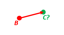
A radar or sonar attached to a vehicle B (Body coordinate frame) measures the distance and direction to an object C. We assume that the distance and two angles (typically bearing and elevation relative to B) are already combined to the vector p_BC_B (i.e. the vector from B to C, decomposed in B). The position of B is given as n_EB_E and z_EB, and the orientation (attitude) of B is given as R_NB (this rotation matrix can be found from roll/pitch/yaw by using zyx2R).

Find the exact position of object C as n-vector and depth ( n_EC_E and z_EC ), assuming Earth ellipsoid with semi-major axis a and flattening f. For WGS-72, use a = 6 378 135 m and f = 1/298.26.

Solution:

>>> import numpy as np
>>> import nvector as nv
>>> wgs72 = nv.FrameE(name="WGS72")
>>> wgs72 = nv.FrameE(a=6378135, f=1.0/298.26)

Step 1: Position and orientation of B is given 400m above E:

>>> n_EB_E = wgs72.Nvector(nv.unit([[1], [2], [3]]), z=-400)
>>> frame_B = nv.FrameB(n_EB_E, yaw=10, pitch=20, roll=30, degrees=True)

Step 2: Delta BC decomposed in B

>>> p_BC_B = frame_B.Pvector(np.r_[3000, 2000, 100].reshape((-1, 1)))

Step 3: Decompose delta BC in E

>>> p_BC_E = p_BC_B.to_ecef_vector()

Step 4: Find point C by adding delta BC to EB

>>> p_EB_E = n_EB_E.to_ecef_vector()
>>> p_EC_E = p_EB_E + p_BC_E
>>> pointC = p_EC_E.to_geo_point()

>>> lat, lon, z = pointC.latlon_deg
>>> msg = "Ex2: PosC: lat, lon = {:4.4f}, {:4.4f} deg,  height = {:4.2f} m"
>>> msg.format(lat, lon, -z)
'Ex2: PosC: lat, lon = 53.3264, 63.4681 deg,  height = 406.01 m'

See also

FrameE, FrameL, FrameN

property R_EN: ndarray[tuple[Any, ...], dtype[floating]]

Rotation matrix to go between E and B frame

classmethod from_point(point: ECEFvector | GeoPoint | Nvector, yaw: ArrayLike = 0, pitch: ArrayLike = 0, roll: ArrayLike = 0, degrees: bool = False) → FrameB

Returns FrameB where its origin coincides with the vehicle’s reference point.

Parameters:

• point (ECEFvector, GeoPoint or Nvector) – Position of the vehicle’s reference point which also coincides with the origin of the frame B.

• yaw (npt.ArrayLike) – Defining the orientation(s) of frame B in [deg] or [rad].

• pitch (npt.ArrayLike) – Defining the orientation(s) of frame B in [deg] or [rad].

• roll (npt.ArrayLike) – Defining the orientation(s) of frame B in [deg] or [rad].

• degrees (bool) – if True yaw, pitch, roll are given in degrees otherwise in radians

class nvector.objects.FrameE(a: float | None = None, f: float | None = None, name: str = 'WGS84', axes: str = 'e')

Earth-fixed frame

a

Semi-major axis of the Earth ellipsoid given in [m].

Type:

float

f

Flattening [no unit] of the Earth ellipsoid. If f==0 then spherical Earth with radius a.

Type:

float

name

Defines the default ellipsoid if not a or f are specified. Default “WGS84”. See get_ellipsoid for valid options.

Type:

str

axes

Either “e” or “E”. Defines axes orientation of E frame. Default is axes=”e” which means that the orientation of the axis is such that: z-axis -> North Pole, x-axis -> Latitude=Longitude=0.

Type:

str

Notes

The frame is Earth-fixed (rotates and moves with the Earth) where the origin coincides with Earth’s centre (geometrical centre of ellipsoid model).

See also

FrameN, FrameL, FrameB, nvector.util.get_ellipsoid

ECEFvector(pvector: List[Any] | Tuple[Any, ...] | ndarray[tuple[Any, ...], dtype[Any]], scalar: bool | None = None) → ECEFvector

Returns ECEFvector from cartesian position vector(s) in current frame.

Parameters:

• pvector (List[Any] | Tuple[Any, ...] | npt.NDArray[Any]) – 3 x n array of cartesian position vector(s) [m] from E to B, decomposed in E.

• scalar (bool) – True if p-vector represents a scalar position, i.e. n = 1.

GeoPoint(latitude: ArrayLike, longitude: ArrayLike, z: ArrayLike = 0, degrees: bool = False) → GeoPoint

Returns GeoPoint from latitude, longitude, depth in current frame.

Parameters:

• latitude (npt.ArrayLike) – Geodetic latitude(s) given in [rad or deg]

• longitude (npt.ArrayLike) – Geodetic longitude(s) given in [rad or deg]

• z (npt.ArrayLike) – Depth(s) [m] relative to the ellipsoid (depth = -height)

• degrees (bool) – True if input are given in degrees otherwise radians are assumed.

GeoPointFromDegrees(latitude: ArrayLike, longitude: ArrayLike, z: ArrayLike = 0) → GeoPoint

Returns GeoPoint from latitude [deg], longitude [deg], depth in current frame

Parameters:

• latitude (npt.ArrayLike) – Geodetic latitude(s) given in [rad or deg]

• longitude (npt.ArrayLike) – Geodetic longitude(s) given in [rad or deg]

• z (npt.ArrayLike) – Depth(s) [m] relative to the ellipsoid (depth = -height)

Nvector(normal: ArrayLike, z: ArrayLike = 0) → Nvector

Returns Nvector from n-vector(s) and depth(s) in current frame.

Parameters:

• normal (List[Any] | Tuple[Any, ...] | npt.NDArray[Any]) – 3 x n array of n-vector(s) [no unit] decomposed in E.

• z (npt.ArrayLike) – Depth(s) [m] relative to the ellipsoid (depth = -height)

property R_Ee: ndarray[tuple[Any, ...], dtype[floating]]

Rotation matrix R_Ee defining the axes of the coordinate frame E

direct(lat_a: ArrayLike, lon_a: ArrayLike, azimuth: ArrayLike, distance: ArrayLike, z: ArrayLike = 0, long_unroll: bool = False, degrees: bool = False) → tuple[floating | ndarray[tuple[Any, ...], dtype[floating]], floating | ndarray[tuple[Any, ...], dtype[floating]], floating | ndarray[tuple[Any, ...], dtype[floating]]]

Returns position B computed from position A, distance and azimuth.

Parameters:

• lat_a (npt.ArrayLike) – Scalar or length n vector of latitude of position A.

• lon_a (npt.ArrayLike) – Scalar or length n vector of longitude of position A.

• azimuth (npt.ArrayLike) – Scalar or length n vector azimuth [rad or deg] of line at position A relative to North.

• distance (npt.ArrayLike) – Scalar or length n vector ellipsoidal distance [m] between position A and B.

• z (npt.ArrayLike) – Scalar or length n vector depth relative to Earth ellipsoid (default = 0).

• long_unroll (bool) – Controls the treatment of longitude. If it is False then the lon_a and lon_b are both reduced to the range [-180, 180). If it is True, then lon_a is as given in the function call and (lon_b - lon_a) determines how many times and in what sense the geodesic has encircled the ellipsoid.

• degrees (bool) – Angles are given in degrees if True otherwise in radians.

Returns:

• lat_b, lon_b (np.floating | npt.NDArray[np.floating]) – Latitude(s) and longitude(s) of position B. (Scalar or vector)

• azimuth_b (np.floating | npt.NDArray[np.floating]) – Azimuth(s) [rad or deg] of line(s) at position B relative to North.

Notes

This method is a thin wrapper around the karney.geodesic.reckon function, which is an implementation of the method described in [Kar13].

Restriction on the parameters:

• Latitudes must lie between -90 and 90 degrees.

• Latitudes outside this range will be set to NaNs.

• The flattening f should be between -1/50 and 1/50 inn order to retain full accuracy.

inverse(lat_a: ArrayLike, lon_a: ArrayLike, lat_b: ArrayLike, lon_b: ArrayLike, z: ArrayLike = 0, degrees: bool = False) → tuple[floating | ndarray[tuple[Any, ...], dtype[floating]], floating | ndarray[tuple[Any, ...], dtype[floating]], floating | ndarray[tuple[Any, ...], dtype[floating]]]

Returns ellipsoidal distance between positions as well as the direction.

Parameters:

• lat_a (npt.ArrayLike) – Scalar or vectors of latitude of position A.

• lon_a (npt.ArrayLike) – Scalar or vectors of longitude of position A.

• lat_b (npt.ArrayLike) – Scalar or vectors of latitude of position B.

• lon_b (npt.ArrayLike) – Scalar or vectors of longitude of position B.

• z (npt.ArrayLike) – Scalar or vectors of depth relative to Earth ellipsoid (default = 0)

• degrees (bool) – Angles are given in degrees if True otherwise in radians.

Returns:

• s_ab (np.floating | npt.NDArray[np.floating]) – Ellipsoidal distance [m] between position A and B.

• azimuth_a, azimuth_b (np.floating | npt.NDArray[np.floating]) – Direction [rad or deg] of line at position A and B relative to North, respectively.

Notes

This method is a thin wrapper around the karney.geodesic.distance function, which is an implementation of the method described in [Kar13].

Restriction on the parameters:

• Latitudes must lie between -90 and 90 degrees.

• Latitudes outside this range will be set to NaNs.

• The flattening f should be between -1/50 and 1/50 inn order to retain full accuracy.

class nvector.objects.FrameL(nvector: Nvector, wander_azimuth: ArrayLike = 0)

Local level, Wander azimuth frame

nvector

Defines the origin of the local frame L. The origin is directly beneath or above the vehicle (B), at the surface of ellipsoid model.

Type:

Nvector

wander_azimuth

Angle(s) [rad] between the x-axis of L and the north direction.

Type:

ndarray

Notes

The Cartesian frame is local and oriented Wander-azimuth-Down. This means that the z-axis is pointing down. Initially, the x-axis points towards north, and the y-axis points towards east, but as the vehicle moves they are not rotating about the z-axis (their angular velocity relative to the Earth has zero component along the z-axis).

(Note: Any initial horizontal direction of the x- and y-axes is valid for L, but if the initial position is outside the poles, north and east are usually chosen for convenience.)

The L-frame is equal to the N-frame except for the rotation about the z-axis, which is always zero for this frame (relative to E). Hence, at a given time, the only difference between the frames is an angle between the x-axis of L and the north direction; this angle is called the wander azimuth angle. The L-frame is well suited for general calculations, as it is non-singular.

See also

FrameE, FrameN, FrameB

property R_EN: ndarray[tuple[Any, ...], dtype[floating]]

Rotation matrix to go between E and L frame

classmethod from_point(point: ECEFvector | GeoPoint | Nvector, wander_azimuth: ArrayLike = 0) → FrameL

Returns FrameL with its origin projected from the point to the surface of ellipsoid model

Parameters:

• point (ECEFvector, GeoPoint or Nvector) – Position of the vehicle (B) which also defines the origin of the local frame L. The origin is directly beneath or above the vehicle (B), at the surface of ellipsoid model.

• wander_azimuth (npt.ArrayLike) – Angle(s) [rad] between the x-axis of L and the north direction.

class nvector.objects.FrameN(nvector: Nvector)

North-East-Down frame

nvector

Defines the origin of the local frame N. The origin is directly beneath or above the vehicle (B), at the surface of ellipsoid model.

Type:

Nvector

Notes

The Cartesian frame is local and oriented North-East-Down, i.e., the x-axis points towards north, the y-axis points towards east (both are horizontal), and the z-axis is pointing down.

When moving relative to the Earth, the frame rotates about its z-axis to allow the x-axis to always point towards north. When getting close to the poles this rotation rate will increase, being infinite at the poles. The poles are thus singularities and the direction of the x- and y-axes are not defined here. Hence, this coordinate frame is NOT SUITABLE for general calculations.

Examples

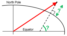
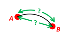
Example 1: “A and B to delta”

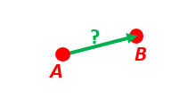
Given two positions, A and B as latitudes, longitudes and depths relative to Earth, E.

Find the exact vector between the two positions, given in meters north, east, and down, and find the direction (azimuth) to B, relative to north, as well as elevation and distance.

Assume WGS-84 ellipsoid. The given depths are from the ellipsoid surface. Use position A to define north, east, and down directions. (Due to the curvature of Earth and different directions to the North Pole, the north, east, and down directions will change (relative to Earth) for different places. Position A must be outside the poles for the north and east directions to be defined.)

Solution:

>>> import numpy as np
>>> import nvector as nv
>>> wgs84 = nv.FrameE(name="WGS84")
>>> pointA = wgs84.GeoPointFromDegrees(latitude=1, longitude=2, z=3)
>>> pointB = wgs84.GeoPointFromDegrees(latitude=4, longitude=5, z=6)

Step1: Find p_AB_N (delta decomposed in N).

>>> p_AB_N = pointA.delta_to(pointB)
>>> x, y, z = p_AB_N.pvector.ravel()
>>> "Ex1: delta north, east, down = {0:8.2f}, {1:8.2f}, {2:8.2f}".format(x, y, z)
'Ex1: delta north, east, down = 331730.23, 332997.87, 17404.27'

Step2: Find the direction (azimuth) to B, relative to north, as well as elevation and distance:

>>> "azimuth = {0:4.2f} deg".format(p_AB_N.azimuth_deg)
'azimuth = 45.11 deg'
>>> "elevation = {0:4.2f} deg".format(p_AB_N.elevation_deg)
'elevation = 2.12 deg'
>>> "distance = {0:4.2f} m".format(p_AB_N.length)
'distance = 470356.72 m'

See also

FrameE, FrameL, FrameB

property R_EN: ndarray[tuple[Any, ...], dtype[floating]]

Rotation matrix to go between E and N frame

classmethod from_point(point: ECEFvector | GeoPoint | Nvector) → FrameN

Returns FrameN with its origin projected from the point to the surface of ellipsoid model

Parameters:

point (ECEFvector, GeoPoint or Nvector) – Position of the vehicle (B) which also defines the origin of the local frame N. The origin is directly beneath or above the vehicle (B), at the surface of ellipsoid model.

class nvector.objects.GeoPath(point_a: Nvector | GeoPoint | ECEFvector, point_b: Nvector | GeoPoint | ECEFvector)

Geographical path between two positions in Frame E

point_a, point_b

The path is defined by the line between position A and B, decomposed in E.

Type:

Nvector, GeoPoint or ECEFvector

Notes

Please note that either position A or B or both might be a vector of points. In this case the GeoPath instance represents all the paths between the positions of A and the corresponding positions of B.

Examples

Example 5: “Surface distance”

Find the surface distance sAB (i.e. great circle distance) between two positions A and B. The heights of A and B are ignored, i.e. if they don’t have zero height, we seek the distance between the points that are at the surface of the Earth, directly above/below A and B. The Euclidean distance (chord length) dAB should also be found. Use Earth radius 6371e3 m. Compare the results with exact calculations for the WGS-84 ellipsoid.

Solution for a sphere:

>>> import numpy as np
>>> import nvector as nv
>>> frame_E = nv.FrameE(a=6371e3, f=0)
>>> pointA = frame_E.GeoPointFromDegrees(latitude=88, longitude=0)
>>> pointB = frame_E.GeoPointFromDegrees(latitude=89, longitude=-170)

>>> s_AB, azia, azib = pointA.distance_and_azimuth(pointB)
>>> p_AB_E = pointB.to_ecef_vector() - pointA.to_ecef_vector()
>>> d_AB = p_AB_E.length

>>> msg = "Ex5: Great circle and Euclidean distance = {}"
>>> msg = msg.format("{:5.2f} km, {:5.2f} km")
>>> msg.format(s_AB / 1000, d_AB / 1000)
'Ex5: Great circle and Euclidean distance = 332.46 km, 332.42 km'

Alternative sphere solution:

>>> path = nv.GeoPath(pointA, pointB)
>>> s_AB2 = path.track_distance(method="greatcircle")
>>> d_AB2 = path.track_distance(method="euclidean")
>>> msg.format(s_AB2 / 1000, d_AB2 / 1000)
'Ex5: Great circle and Euclidean distance = 332.46 km, 332.42 km'

Exact solution for the WGS84 ellipsoid:

>>> wgs84 = nv.FrameE(name="WGS84")
>>> point1 = wgs84.GeoPointFromDegrees(latitude=88, longitude=0)
>>> point2 = wgs84.GeoPointFromDegrees(latitude=89, longitude=-170)
>>> s_12, azi1, azi2 = point1.distance_and_azimuth(point2)

>>> p_12_E = point2.to_ecef_vector() - point1.to_ecef_vector()
>>> d_12 = p_12_E.length
>>> msg = "Ellipsoidal and Euclidean distance = {:5.2f} km, {:5.2f} km"
>>> msg.format(s_12 / 1000, d_12 / 1000)
'Ellipsoidal and Euclidean distance = 333.95 km, 333.91 km'

Example 6 “Interpolated position”

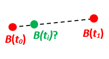
Given the position of B at time t0 and t1, n_EB_E(t0) and n_EB_E(t1).

Find an interpolated position at time ti, n_EB_E(ti). All positions are given as n-vectors.

Solution:

>>> import nvector as nv
>>> wgs84 = nv.FrameE(name="WGS84")
>>> n_EB_E_t0 = wgs84.GeoPointFromDegrees(89, 0).to_nvector()
>>> n_EB_E_t1 = wgs84.GeoPointFromDegrees(89, 180).to_nvector()
>>> path = nv.GeoPath(n_EB_E_t0, n_EB_E_t1)

>>> t0 = 10.
>>> t1 = 20.
>>> ti = 16.  # time of interpolation
>>> ti_n = (ti - t0) / (t1 - t0) # normalized time of interpolation

>>> g_EB_E_ti = path.interpolate(ti_n).to_geo_point()

>>> lat_ti, lon_ti, z_ti = g_EB_E_ti.latlon_deg
>>> msg = "Ex6, Interpolated position: lat, lon = {:2.1f} deg, {:2.1f} deg"
>>> msg.format(lat_ti, lon_ti)
'Ex6, Interpolated position: lat, lon = 89.8 deg, 180.0 deg'

Vectorized solution:

>>> t = np.array([10, 20])
>>> nvectors = wgs84.GeoPointFromDegrees([89, 89], [0, 180]).to_nvector()
>>> nvectors_i = nvectors.interpolate(ti, t, kind="linear")
>>> lati, loni, zi = nvectors_i.to_geo_point().latlon_deg
>>> msg.format(lat_ti, lon_ti)
'Ex6, Interpolated position: lat, lon = 89.8 deg, 180.0 deg'

Example 9: “Intersection of two paths”

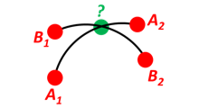
Define a path from two given positions (at the surface of a spherical Earth), as the great circle that goes through the two points.

Path A is given by A1 and A2, while path B is given by B1 and B2.

Find the position C where the two great circles intersect.

Solution:

>>> import nvector as nv
>>> pointA1 = nv.GeoPoint.from_degrees(10, 20)
>>> pointA2 = nv.GeoPoint.from_degrees(30, 40)
>>> pointB1 = nv.GeoPoint.from_degrees(50, 60)
>>> pointB2 = nv.GeoPoint.from_degrees(70, 80)
>>> pathA = nv.GeoPath(pointA1, pointA2)
>>> pathB = nv.GeoPath(pointB1, pointB2)

>>> pointC = pathA.intersect(pathB)
>>> pointC = pointC.to_geo_point()
>>> lat, lon = pointC.latitude_deg, pointC.longitude_deg
>>> msg = "Ex9, Intersection: lat, lon = {:4.4f}, {:4.4f} deg"
>>> msg.format(lat, lon)
'Ex9, Intersection: lat, lon = 40.3186, 55.9019 deg'

Check that PointC is not between A1 and A2 or B1 and B2:

>>> bool(pathA.on_path(pointC))
False
>>> bool(pathB.on_path(pointC))
False

Check that PointC is on the great circle going through path A and path B:

>>> bool(pathA.on_great_circle(pointC))
True
>>> bool(pathB.on_great_circle(pointC))
True

Example 10: “Cross track distance”

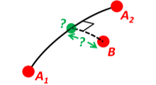
Path A is given by the two positions A1 and A2 (similar to the previous example).

Find the cross track distance sxt between the path A (i.e. the great circle through A1 and A2) and the position B (i.e. the shortest distance at the surface, between the great circle and B).

Also find the Euclidean distance dxt between B and the plane defined by the great circle. Use Earth radius 6371e3.

Finally, find the intersection point on the great circle and determine if it is between position A1 and A2.

Solution:

>>> import numpy as np
>>> import nvector as nv
>>> frame = nv.FrameE(a=6371e3, f=0)
>>> pointA1 = frame.GeoPoint(0, 0)
>>> pointA2 = frame.GeoPointFromDegrees(10, 0)
>>> pointB = frame.GeoPointFromDegrees(1, 0.1)
>>> pathA = nv.GeoPath(pointA1, pointA2)

>>> s_xt = pathA.cross_track_distance(pointB, method="greatcircle")
>>> d_xt = pathA.cross_track_distance(pointB, method="euclidean")

>>> val_txt = "{:4.2f} km, {:4.2f} km".format(s_xt/1000, d_xt/1000)
>>> "Ex10: Cross track distance: s_xt, d_xt = {}".format(val_txt)
'Ex10: Cross track distance: s_xt, d_xt = 11.12 km, 11.12 km'

>>> pointC = pathA.closest_point_on_great_circle(pointB)
>>> bool(np.allclose(pathA.on_path(pointC), True))
True

closest_point_on_great_circle(point: Nvector | GeoPoint | ECEFvector) → GeoPoint

Returns closest point on great circle path to the point.

Parameters:

point (GeoPoint, Nvector or ECEFvector) – Point of intersection between paths

Returns:

closest_point – Closest point on path.

Return type:

GeoPoint

Notes

The result for spherical Earth is returned at the average depth.

Examples

>>> import nvector as nv
>>> wgs84 = nv.FrameE(name="WGS84")
>>> point_a = wgs84.GeoPoint(51., 1., degrees=True)
>>> point_b = wgs84.GeoPoint(51., 2., degrees=True)
>>> point_c = wgs84.GeoPoint(51., 2.9, degrees=True)
>>> path = nv.GeoPath(point_a, point_b)
>>> point = path.closest_point_on_great_circle(point_c)
>>> bool(path.on_path(point))
False
>>> bool(nv.allclose((point.latitude_deg, point.longitude_deg),
...                  (50.99270338, 2.89977984)))
True

>>> bool(nv.allclose(GeoPath(point_c, point).track_distance(),  810.76312076))
True

closest_point_on_path(point: Nvector | GeoPoint | ECEFvector) → GeoPoint

Returns closest point on great circle path segment to the point.

If the point is within the extent of the segment, the point returned is on the segment path otherwise, it is the closest endpoint defining the path segment.

Parameters:

point (GeoPoint) – Point of intersection between paths

Returns:

closest_point – Closest point on path segment.

Return type:

GeoPoint

Examples

>>> import nvector as nv
>>> wgs84 = nv.FrameE(name="WGS84")
>>> pointA = wgs84.GeoPoint(51., 1., degrees=True)
>>> pointB = wgs84.GeoPoint(51., 2., degrees=True)
>>> pointC = wgs84.GeoPoint(51., 1.9, degrees=True)
>>> path = nv.GeoPath(pointA, pointB)
>>> point = path.closest_point_on_path(pointC)
>>> bool(np.allclose((point.latitude_deg, point.longitude_deg),
...                  (51.00038411380564, 1.900003311624411)))
True
>>> bool(np.allclose(GeoPath(pointC, point).track_distance(),  42.67368351))
True
>>> pointD = wgs84.GeoPoint(51.0, 2.1, degrees=True)
>>> pointE = path.closest_point_on_path(pointD) # 51.0000, 002.0000
>>> float(pointE.latitude_deg), float(pointE.longitude_deg)
(51.0, 2.0)

cross_track_distance(point: Nvector | GeoPoint | ECEFvector, method: str = 'greatcircle', radius: floating | ndarray[tuple[Any, ...], dtype[floating]] | None = None) → floating | ndarray[tuple[Any, ...], dtype[floating]]

Returns cross track distance from path to point.

Parameters:

• point (GeoPoint, Nvector or ECEFvector) – Position(s) to measure the cross track distance to.

• method (str) – Either “greatcircle” or “euclidean” defining distance calculated.

• radius (real scalar) – Radius of sphere in [m]. Default is the average height of points A and B.

Returns:

distance – Distance(s) in [m]

Return type:

real scalar or vector

Notes

The result for spherical Earth is returned.

ecef_vectors() → tuple[ECEFvector, ECEFvector]

Returns point A and point B as ECEF-vectors

geo_points() → tuple[GeoPoint, GeoPoint]

Returns point A and point B as geo-points

interpolate(ti: ArrayLike) → Nvector

Returns the interpolated point along the path

Parameters:

ti (npt.ArrayLike) – Interpolation time(s) assuming position A and B is at t0=0 and t1=1, respectively.

Returns:

point – Point of interpolation along path

Return type:

Nvector

intersect(path: GeoPath) → Nvector

Returns the intersection(s) between the great circles of the two paths

Parameters:

path (GeoPath) – Path to intersect

Returns:

point – Intersection(s) between the great circles of the two paths

Return type:

Nvector

Notes

The result for spherical Earth is returned at the average height.

nvector_normals() → tuple[ndarray[tuple[Any, ...], dtype[floating]], ndarray[tuple[Any, ...], dtype[floating]]]

Returns nvector normals for position a and b

nvectors() → tuple[Nvector, Nvector]

Returns point A and point B as n-vectors

on_great_circle(point: Nvector | GeoPoint | ECEFvector, atol: float = 1e-08) → bool | ndarray[tuple[Any, ...], dtype[bool]]

Returns True if point is on the great circle within a tolerance.

on_path(point: Nvector | GeoPoint | ECEFvector, method: str = 'greatcircle', rtol: float = 1e-06, atol: float = 1e-08) → ndarray[tuple[Any, ...], dtype[bool]]

Returns True if point is on the path between A and B witin a tolerance.

Parameters:

• point (Nvector, GeoPoint or ECEFvector) – Point to test

• method ("greatcircle" or "ellipsoid") – Defines the path.

• rtol (real scalar) – The relative tolerance parameter.

• atol (real scalar) – The absolute tolerance parameter.

Returns:

result – True if the point is on the path at its average height.

Return type:

Boolean vector

Notes

The result for spherical Earth is returned for method=”greatcircle”.

Examples

>>> import nvector as nv
>>> wgs84 = nv.FrameE(name="WGS84")
>>> pointA = wgs84.GeoPointFromDegrees(89, 0)
>>> pointB = wgs84.GeoPointFromDegrees(80, 0)
>>> path = nv.GeoPath(pointA, pointB)
>>> pointC = path.interpolate(0.6).to_geo_point()
>>> bool(path.on_path(pointC))
True
>>> bool(path.on_path(pointC, "ellipsoid"))
True
>>> pointD = path.interpolate(1.000000001).to_geo_point()
>>> bool(path.on_path(pointD))
False
>>> bool(path.on_path(pointD, "ellipsoid"))
False
>>> pointE = wgs84.GeoPointFromDegrees(85, 0.0001)
>>> bool(path.on_path(pointE))
False
>>> pointC = path.interpolate(-2).to_geo_point()
>>> bool(path.on_path(pointC))
False
>>> bool(path.on_great_circle(pointC))
True

track_distance(method: str = 'greatcircle', radius: float | None = None) → floating | ndarray[tuple[Any, ...], dtype[floating]]

Returns the path distance computed at the average height in [m].

Parameters:

• method (str) – “greatcircle”, “euclidean” or “ellipsoidal” defining distance calculated.

• radius (real scalar) – Radius of sphere. Default is the average height of points A and B

class nvector.objects.GeoPoint(latitude: ArrayLike, longitude: ArrayLike, z: ArrayLike = 0, frame: FrameE | None = None, degrees: bool = False)

Geographical position(s) given as latitude(s), longitude(s), depth(s) in frame E.

latitude, longitude

Geodetic latitude(s) and longitude(s) given in [rad]

Type:

ndarray

z

Depth(s) [m] relative to the ellipsoid (depth = -height)

Type:

ndarray

frame

Reference ellipsoid. The default ellipsoid model used is WGS84, but other ellipsoids/spheres might be specified.

Type:

FrameE

Notes

Please note that latitude, longitude and z are broadcasted together in the __init__ function. If either one of them is a vector the GeoPoint instance then will represents multiple positions.

Examples

Solve geodesic problems.

The following illustrates its use

>>> import nvector as nv
>>> wgs84 = nv.FrameE(name="WGS84")
>>> point_a = wgs84.GeoPointFromDegrees(-41.32, 174.81)
>>> point_b = wgs84.GeoPointFromDegrees(40.96, -5.50)

>>> print(point_a)
GeoPoint(
    latitude=-0.721170046924057,
    longitude=3.0510100654112877,
    z=0,
    frame=FrameE(a=6378137.0, f=0.0033528106647474805, name='WGS84', axes='e'))

The geodesic inverse problem

>>> s12, az1, az2 = point_a.distance_and_azimuth(point_b, degrees=True)
>>> "s12 = {:5.2f}, az1 = {:5.2f}, az2 = {:5.2f}".format(s12, az1, az2)
's12 = 19959679.27, az1 = 161.07, az2 = 18.83'

The geodesic direct problem

>>> point_a = wgs84.GeoPointFromDegrees(40.6, -73.8)
>>> az1, distance = 45, 10000e3
>>> point_b, az2 = point_a.displace(distance, az1, degrees=True)
>>> lat2, lon2 = point_b.latitude_deg, point_b.longitude_deg
>>> msg = "lat2 = {:5.2f}, lon2 = {:5.2f}, az2 = {:5.2f}"
>>> msg.format(lat2, lon2, az2)
'lat2 = 32.64, lon2 = 49.01, az2 = 140.37'

delta_to(other: Nvector | GeoPoint | ECEFvector) → Pvector

Returns cartesian delta vector from current position to the other decomposed in N.

Parameters:

other (Nvector, GeoPoint or ECEFvector) – Other position decomposed in E.

Returns:

p_AB_N – Delta vector from current position (A) to the other position (B), decomposed in N.

Return type:

Pvector

displace(distance: ArrayLike, azimuth: ArrayLike, long_unroll: bool = False, degrees: bool = False, method: str = 'ellipsoid') → tuple[GeoPoint, floating | ndarray[tuple[Any, ...], dtype[floating]]]

Returns position b computed from current position, distance and azimuth.

Parameters:

• distance (npt.ArrayLike) – Ellipsoidal or great circle distance(s) [m] between positions A and B.

• azimuth (npt.ArrayLike) – Azimuth(s) [rad or deg] of line(s) at position A.

• long_unroll (bool) – Controls the treatment of longitude when method==”ellipsoid”. See distance_and_azimuth method for details.

• degrees (bool) – azimuths are given in degrees if True otherwise in radians.

• method (str) – Either “greatcircle” or “ellipsoid”, defining the path where to find position B.

Returns:

• point_b (GeoPoint) – B position(s).

• azimuth_b (float64 or ndarray) – Azimuth(s) [rad or deg] of line(s) at position(s) B.

Notes

The karney.geodesic.reckon function is used When the method is “ellipsoid”. Keep for full double precision accuracy in this case. See [Kar13] for a description of the method.

distance_and_azimuth(point: GeoPoint | Nvector | ECEFvector | Pvector, degrees: bool = False, method: str = 'ellipsoid') → tuple[floating | ndarray[tuple[Any, ...], dtype[floating]], floating | ndarray[tuple[Any, ...], dtype[floating]], floating | ndarray[tuple[Any, ...], dtype[floating]]]

Returns ellipsoidal distance between positions as well as the direction.

Parameters:

• point (GeoPoint, Nvector, ECEFvector or Pvector) – Geographical position(s) B.

• degrees (bool) – Azimuths are returned in degrees if True otherwise in radians.

• method (str) – Either “greatcircle” or “ellipsoid” defining the path distance calculated.

Returns:

• s_ab (float64 or ndarray) – Ellipsoidal distance(s) [m] between A and B position(s) at their average height.

• azimuth_a, azimuth_b (float64 or ndarray) – Direction(s) [rad or deg] of line(s) at position A and B relative to North, respectively.

Notes

The karney.geodesic.distance function is used When the method is “ellipsoid”. Keep for full double precision accuracy in this case. See [Kar13] for a description of the method.

Examples

>>> import nvector as nv
>>> point1 = nv.GeoPoint(0, 0)
>>> point2 = nv.GeoPoint.from_degrees(0.5, 179.5)
>>> s_12, az1, azi2 = point1.distance_and_azimuth(point2)
>>> bool(nv.allclose(s_12, 19936288.579))
True

classmethod from_degrees(latitude: ArrayLike, longitude: ArrayLike, z: ArrayLike = 0, frame: FrameE | None = None) → GeoPoint

Returns GeoPoint from latitude [deg], longitude [deg], depth in frame E.

Parameters:

• latitude (npt.ArrayLike) – Geodetic latitude(s) [deg] (scalar or vector)

• longitude (npt.ArrayLike) – Geodetic longitude(s) [deg] (scalar or vector)

• z (npt.ArrayLike) – Depth(s) [m] relative to the ellipsoid. (depth = -height) (scalar or vector)

• frame (FrameE) – Reference ellipsoid. The default ellipsoid model used is WGS84, but other ellipsoids/spheres might be specified.

property latitude_deg: ndarray[tuple[Any, ...], dtype[floating]]

Latitude in degrees.

property latlon: tuple[ndarray[tuple[Any, ...], dtype[floating]], ndarray[tuple[Any, ...], dtype[floating]], ndarray[tuple[Any, ...], dtype[floating]]]

Latitude [rad], longitude [rad], and depth [m].

property latlon_deg: tuple[ndarray[tuple[Any, ...], dtype[floating]], ndarray[tuple[Any, ...], dtype[floating]], ndarray[tuple[Any, ...], dtype[floating]]]

Latitude [deg], longitude [deg] and depth [m].

property longitude_deg: ndarray[tuple[Any, ...], dtype[floating]]

Longitude in degrees.

property scalar: bool

True if the position is a scalar point

to_ecef_vector() → ECEFvector

Returns position(s) as ECEFvector object.

to_geo_point() → GeoPoint

Returns position(s) as GeoPoint object, in this case, itself.

to_nvector() → Nvector

Returns position(s) as Nvector object.

class nvector.objects.Nvector(normal: ArrayLike, z: ArrayLike = 0, frame: FrameE | None = None)

Geographical position(s) given as n-vector(s) and depth(s) in frame E

normal

Normal vector(s) [no unit] decomposed in E.

Type:

ndarray

z

Depth(s) [m] relative to the ellipsoid. (depth = -height)

Type:

ndarray

frame

Reference ellipsoid. The default ellipsoid model used is WGS84, but other ellipsoids/spheres might be specified.

Type:

FrameE

Notes

The position of B (typically body) relative to E (typically Earth) is given into this function as n-vector, n_EB_E and a depth, z relative to the ellipsiod.

Examples

>>> import nvector as nv
>>> wgs84 = nv.FrameE(name="WGS84")
>>> point_a = wgs84.GeoPointFromDegrees(-41.32, 174.81)
>>> point_b = wgs84.GeoPointFromDegrees(40.96, -5.50)
>>> nv_a = point_a.to_nvector()
>>> print(nv_a)
Nvector(
    normal=[[-0.74795462]
            [ 0.06793758]
            [-0.66026387]],
    z=[0],
    frame=FrameE(a=6378137.0, f=0.0033528106647474805, name='WGS84', axes='e'))

See also

GeoPoint, ECEFvector, Pvector

__mul__(scalar: Any) → Nvector

Elementwise multiplication

__rmul__(scalar: Any) → Nvector

Elementwise multiplication

__truediv__(scalar: Any) → Nvector

Elementwise division

course_over_ground(**options: Any) → floating | ndarray[tuple[Any, ...], dtype[floating]]

Returns course over ground in radians from nvector positions

Parameters:

**options (dict) –

Optional keyword arguments to apply a Savitzky-Golay smoothing filter window. No smoothing is applied by default. Valid keyword arguments are:

window_length: int

The length of the Savitzky-Golay filter window (i.e., the number of coefficients). Positive odd integer or zero. Default window_length=0, i.e. no smoothing.

polyorder: int

The order of the polynomial used to fit the samples. The value must be less than window_length. Default is 2.

mode: str

Valid options are: “mirror”, “constant”, “nearest”, “wrap” or “interp”. Determines the type of extension to use for the padded signal to which the filter is applied. When mode is “constant”, the padding value is given by cval. When the “nearest” mode is selected (the default) the extension contains the nearest input value. When the “interp” mode is selected, no extension is used. Instead, a degree polyorder polynomial is fit to the last window_length values of the edges, and this polynomial is used to evaluate the last window_length // 2 output values. Default “nearest”.

cval: int or float

Value to fill past the edges of the input if mode is “constant”. Default is 0.0.

Returns:

cog – Angle(s) in radians clockwise from True North to the direction towards which the vehicle travels. If n<2 NaN is returned.

Return type:

np.floating | npt.NDArray[np.floating]

Notes

Please be aware that this method requires the vehicle positions to be very smooth! If they are not you should probably smooth it by a window_length corresponding to a few seconds or so. The smoothing filter is only applied if the optional keyword window_length value is an integer and >0. Also note that at least n>=2 points are needed to obtain meaningful results.

See https://www.navlab.net/Publications/The_Seven_Ways_to_Find_Heading.pdf for an overview of methods to find accurate headings.

Examples

>>> import matplotlib.pyplot as plt
>>> import nvector as nv
>>> points = nv.GeoPoint.from_degrees((59.381509, 59.387647),(10.496590, 10.494713))
>>> nvec = points.to_nvector()
>>> COG_rad = nvec.course_over_ground()
>>> dx, dy = np.sin(COG_rad[0]), np.cos(COG_rad[0])
>>> COG = nv.deg(COG_rad[0])
>>> p_AB_N = nv.n_EA_E_and_n_EB_E2p_AB_N(nvec.normal[:, :1], nvec.normal[:, 1:]).ravel()
>>> ax = plt.figure().gca()
>>> _ = ax.plot(0, 0, "bo", label="A")
>>> _ = ax.arrow(0,0, dx*300, dy*300, head_width=20)
>>> _ = ax.plot(p_AB_N[1], p_AB_N[0], "go", label="B")
>>> _ = ax.set_title("COG=%2.1f degrees" % COG)
>>> _ = ax.set_xlabel("East [m]")
>>> _ = ax.set_ylabel("North [m]")
>>> _ = ax.set_xlim(-500, 200)
>>> _ = ax.set_aspect("equal", adjustable="box")
>>> _ = ax.legend()
>>> plt.show()
>>> plt.close()

See also

nvector.core.course_over_ground

delta_to(other: Nvector | GeoPoint | ECEFvector) → Pvector

Returns cartesian delta vector from current position to the other decomposed in N.

Parameters:

other (Nvector, GeoPoint or ECEFvector) – Other position decomposed in E.

Returns:

p_AB_N – Delta vector from current position (A) to the other position (B), decomposed in N.

Return type:

Pvector

interpolate(t_i: ArrayLike, t: ArrayLike, kind: int | str = 'linear', window_length: int = 0, polyorder: int = 2, mode: str = 'interp', cval: int | float = 0.0) → Nvector

Returns interpolated values from nvector data.

Parameters:

• t_i (npt.ArrayLike) – Real vector of length m. Vector of interpolation times.

• t (List[Any] | Tuple[Any, ...] | npt.NDArray[Any]) – Real vector of length n. Vector of times.

• kind (str or int) – Specifies the kind of interpolation as a string (“linear”, “nearest”, “zero”, “slinear”, “quadratic”, “cubic” where “zero”, “slinear”, “quadratic” and “cubic” refer to a spline interpolation of zeroth, first, second or third order) or as an integer specifying the order of the spline interpolator to use. Default is “linear”.

• window_length (int) – The length of the Savitzky-Golay filter window (i.e., the number of coefficients). Must be positive odd integer or zero. Default window_length=0, i.e. no smoothing.

• polyorder (int) – The order of the polynomial used to fit the samples. polyorder must be less than window_length.

• mode (str) – Accepted values are “mirror”, “constant”, “nearest”, “wrap” or “interp”. Determines the type of extension to use for the padded signal to which the filter is applied. When mode is “constant”, the padding value is given by cval. When the “interp” mode is selected (the default), no extension is used. Instead, a degree polyorder polynomial is fit to the last window_length values of the edges, and this polynomial is used to evaluate the last window_length // 2 output values.

• cval (int or float) – Value to fill past the edges of the input if mode is “constant”. Default is 0.0.

Returns:

Interpolated n-vector(s) [no unit] decomposed in E.

Return type:

Nvector

Notes

The result for spherical Earth is returned.

Examples

>>> import matplotlib.pyplot as plt
>>> import numpy as np
>>> import nvector as nv
>>> lat = np.arange(0, 10)
>>> lon = nv.deg(np.sin(nv.rad(np.linspace(-90, 70, 10))))
>>> nvectors = nv.GeoPoint.from_degrees(lat, lon).to_nvector()
>>> t = np.arange(10)
>>> t_i = np.linspace(0, t[-1], 100)
>>> nvectors_i = nvectors.interpolate(t_i, t, kind="cubic")
>>> lati, loni, zi = nvectors_i.to_geo_point().latlon_deg
>>> h = plt.plot(lon, lat, "o", loni, lati, "-")
>>> plt.show()
>>> plt.close()

mean() → Nvector

Returns the mean position of the n-vectors.

property scalar: bool

True if the position is a scalar point

to_ecef_vector() → ECEFvector

Returns position(s) as ECEFvector object.

to_geo_point() → GeoPoint

Returns position(s) as GeoPoint object.

to_nvector() → Nvector

Returns position(s) as Nvector object, in this case, itself.

unit() → None

Normalizes self to unit vector(s)

class nvector.objects.Pvector(pvector: List[Any] | Tuple[Any, ...] | ndarray[tuple[Any, ...], dtype[Any]], frame: FrameN | FrameB | FrameL | _LocalFrameBase, scalar: bool | None = None)

Geographical position(s) given as cartesian position vector(s) in a frame.

pvector

3 x n array cartesian position vector(s) [m] from E to B, decomposed in E.

Type:

ndarray

frame

Local frame

Type:

FrameN, FrameB or FrameL

scalar

True if p-vector represents a scalar position, i.e. n = 1.

Type:

bool

pvector: ndarray[tuple[Any, ...], dtype[floating]]

Position array-like, must be shape (3, n, m, …) with n>0

to_ecef_vector() → ECEFvector

Returns position(s) as ECEFvector object.

to_geo_point() → GeoPoint

Returns position(s) as GeoPoint object.

to_nvector() → Nvector

Returns position(s) as Nvector object.

nvector.objects.delta_E(point_a: Nvector | GeoPoint | ECEFvector, point_b: Nvector | GeoPoint | ECEFvector) → ECEFvector

Returns cartesian delta vector from positions A to B decomposed in E.

Parameters:

• point_a (Nvector, GeoPoint or ECEFvector) – Position A decomposed in E.

• point_b (Nvector, GeoPoint or ECEFvector) – Position B decomposed in E.

Returns:

p_AB_E – Cartesian position vector(s) from A to B, decomposed in E.

Return type:

ECEFvector

Notes

The calculation is exact, taking the ellipsity of the Earth into account. It is also non-singular as both n-vector and p-vector are non-singular (except for the center of the Earth).

Examples

Example 1: “A and B to delta”

Given two positions, A and B as latitudes, longitudes and depths relative to Earth, E.

Find the exact vector between the two positions, given in meters north, east, and down, and find the direction (azimuth) to B, relative to north, as well as elevation and distance.

Assume WGS-84 ellipsoid. The given depths are from the ellipsoid surface. Use position A to define north, east, and down directions. (Due to the curvature of Earth and different directions to the North Pole, the north, east, and down directions will change (relative to Earth) for different places. Position A must be outside the poles for the north and east directions to be defined.)

Solution:

>>> import numpy as np
>>> import nvector as nv
>>> wgs84 = nv.FrameE(name="WGS84")
>>> pointA = wgs84.GeoPointFromDegrees(latitude=1, longitude=2, z=3)
>>> pointB = wgs84.GeoPointFromDegrees(latitude=4, longitude=5, z=6)

Step1: Find p_AB_N (delta decomposed in N).

>>> p_AB_N = pointA.delta_to(pointB)
>>> x, y, z = p_AB_N.pvector.ravel()
>>> "Ex1: delta north, east, down = {0:8.2f}, {1:8.2f}, {2:8.2f}".format(x, y, z)
'Ex1: delta north, east, down = 331730.23, 332997.87, 17404.27'

Step2: Find the direction (azimuth) to B, relative to north, as well as elevation and distance:

>>> "azimuth = {0:4.2f} deg".format(p_AB_N.azimuth_deg)
'azimuth = 45.11 deg'
>>> "elevation = {0:4.2f} deg".format(p_AB_N.elevation_deg)
'elevation = 2.12 deg'
>>> "distance = {0:4.2f} m".format(p_AB_N.length)
'distance = 470356.72 m'

See also

nvector.core.n_EA_E_and_p_AB_E2n_EB_E, nvector.core.p_EB_E2n_EB_E, nvector.core.n_EB_E2p_EB_E

nvector.objects.delta_L(point_a: Nvector | GeoPoint | ECEFvector, point_b: Nvector | GeoPoint | ECEFvector, wander_azimuth: int | float = 0) → Pvector

Returns cartesian delta vector from positions A to B decomposed in L.

Parameters:

• point_a (Nvector, GeoPoint or ECEFvector) – Position A decomposed in E.

• point_b (Nvector, GeoPoint or ECEFvector) – Position B decomposed in E.

• wander_azimuth (real scalar) – Angle [rad] between the x-axis of L and the north direction.

Returns:

p_AB_L – Cartesian delta vector from positions A to B decomposed in L.

Return type:

Pvector

See also

delta_E, delta_N

nvector.objects.delta_N(point_a: Nvector | GeoPoint | ECEFvector, point_b: Nvector | GeoPoint | ECEFvector) → Pvector

Returns cartesian delta vector from positions A to B decomposed in N.

Parameters:

• point_a (Nvector, GeoPoint or ECEFvector) – Position A decomposed in E.

• point_b (Nvector, GeoPoint or ECEFvector) – Position B decomposed in E.

Returns:

p_AB_N – Delta vector from positions A to B, decomposed in N.

Return type:

Pvector

See also

delta_E, delta_L

5.2. Core geodesic functions

This file is part of NavLab and is available from www.navlab.net/nvector

5.2.1. Functions in module

closest_point_on_great_circle:

Returns closest point C on great circle path A to position B.

cross_track_distance:

Returns cross track distance between path A and position B.

course_over_ground:

Returns course over ground in radians from nvector positions.

euclidean_distance:

Returns Euclidean distance between positions A and B on a sphere.

geodesic_distance:

Returns surface distance between positions A and B on an ellipsoid.

geodesic_reckon:

Returns position B computed from position A, distance and azimuth.

great_circle_distance:

Returns great circle distance between positions A and B on a sphere

great_circle_distance_rad:

Returns great circle distance in radians between positions A and B on a sphere

great_circle_normal:

Returns the unit normal(s) to the great circle(s)

interp_nvectors:

Returns interpolated values from nvector data.

interpolate:

Returns the interpolated point(s) along the path

intersect:

Returns the intersection(s) between the great circles of the two paths

mean_horizontal_position:

Returns the n-vector of the horizontal mean position.

lat_lon2n_E:

Converts latitude and longitude to n-vector.

n_E2lat_lon:

Converts n-vector(s) to latitude(s) and longitude(s).

n_EA_E_and_n_EB_E2p_AB_E:

Returns the delta vector from position A to B decomposed in E.

n_EA_E_and_n_EB_E2p_AB_N:

Returns the delta vector from position A to B decomposed in N.

n_EA_E_and_p_AB_E2n_EB_E:

Returns position B from position A and delta vector decomposed in E.

n_EA_E_and_p_AB_N2n_EB_E:

Returns position B from position A and delta vector decomposed in N.

n_EB_E2p_EB_E:

Converts n-vector to Cartesian position vector in meters.

p_EB_E2n_EB_E:

Converts Cartesian position vector in meters to n-vector.

n_EA_E_distance_and_azimuth2n_EB_E:

Returns position B from azimuth and distance from position A

n_EA_E_and_n_EB_E2azimuth:

Returns azimuth from A to B, relative to North:

on_great_circle:

Returns True if position B is on great circle through path A.

on_great_circle_path:

Returns True if position B is on great circle and between endpoints of path A.

nvector.core.closest_point_on_great_circle(path: Tuple[List[Any] | Tuple[Any, ...] | ndarray[tuple[Any, ...], dtype[Any]], List[Any] | Tuple[Any, ...] | ndarray[tuple[Any, ...], dtype[Any]]], n_EB_E: List[Any] | Tuple[Any, ...] | ndarray[tuple[Any, ...], dtype[Any]]) → ndarray[tuple[Any, ...], dtype[floating]]

Returns closest point C on great circle path A to position B.

Parameters:

• path (tuple[List[Any] | Tuple[Any, ...] | npt.NDArray[Any], List[Any] | Tuple[Any, ...] | npt.NDArray[Any]]) – 2-tuple of n-vectors of shapes 3 x k and 3 x m, respectively, defining path A, decomposed in E.

• n_EB_E (List[Any] | Tuple[Any, ...] | npt.NDArray[Any]) – 3 x n array n-vector(s) of position B to find the closest point to.

Returns:

n_EC_E – 3 x max(k, m, n) array n-vector(s) of closest position C on great circle path A

Return type:

npt.NDArray[np.floating]

Notes

The shape of the output n_EC_E is the broadcasted shapes of n_EB_E and the n-vectors defining path A.

Examples

Example 10: “Cross track distance”

Path A is given by the two positions A1 and A2 (similar to the previous example).

Find the cross track distance sxt between the path A (i.e. the great circle through A1 and A2) and the position B (i.e. the shortest distance at the surface, between the great circle and B).

Also find the Euclidean distance dxt between B and the plane defined by the great circle. Use Earth radius 6371e3.

Finally, find the intersection point on the great circle and determine if it is between position A1 and A2.

Solution:

>>> import numpy as np
>>> import nvector as nv
>>> from nvector import rad, deg
>>> n_EA1_E = nv.lat_lon2n_E(rad(0), rad(0))
>>> n_EA2_E = nv.lat_lon2n_E(rad(10), rad(0))
>>> n_EB_E = nv.lat_lon2n_E(rad(1), rad(0.1))
>>> path = (n_EA1_E, n_EA2_E)
>>> radius = 6371e3  # mean earth radius [m]
>>> s_xt = nv.cross_track_distance(path, n_EB_E, radius=radius)
>>> d_xt = nv.cross_track_distance(path, n_EB_E, method="euclidean",
...                                radius=radius)

>>> val_txt = "{:4.2f} km, {:4.2f} km".format(s_xt[0]/1000, d_xt[0]/1000)
>>> "Ex10: Cross track distance: s_xt, d_xt = {0}".format(val_txt)
'Ex10: Cross track distance: s_xt, d_xt = 11.12 km, 11.12 km'

>>> n_EC_E = nv.closest_point_on_great_circle(path, n_EB_E)
>>> bool(np.allclose(nv.on_great_circle_path(path, n_EC_E, radius), True))
True

Alternative solution 2:

>>> s_xt2 = nv.great_circle_distance(n_EB_E, n_EC_E, radius)
>>> d_xt2 = nv.euclidean_distance(n_EB_E, n_EC_E, radius)
>>> bool(np.allclose(s_xt, s_xt2)), bool(np.allclose(d_xt, d_xt2))
(True, True)

Alternative solution 3:

>>> c_E = nv.great_circle_normal(n_EA1_E, n_EA2_E)
>>> sin_theta = -np.dot(c_E.T, n_EB_E).ravel()
>>> s_xt3 = np.arcsin(sin_theta) * radius
>>> d_xt3 = sin_theta * radius
>>> bool(np.allclose(s_xt, s_xt3)), bool(np.allclose(d_xt, d_xt3))
(True, True)

See also

cross_track_distance, great_circle_normal

nvector.core.course_over_ground(nvectors: List[Any] | Tuple[Any, ...] | ndarray[tuple[Any, ...], dtype[Any]], a: float = 6378137.0, f: float = 0.0033528106647474805, R_Ee: List[Any] | Tuple[Any, ...] | ndarray[tuple[Any, ...], dtype[Any]] | None = None, **options: Any) → floating | ndarray[tuple[Any, ...], dtype[floating]]

Returns course over ground in radians from nvector positions.

Parameters:

• nvectors (npt.ArrayLike) – 3 x n array positions of vehicle given as n-vectors [no unit] decomposed in E.

• a (float) – Semi-major axis of the Earth ellipsoid given in [m], default WGS-84 ellipsoid.

• f (float) – Flattening [no unit] of the Earth ellipsoid, default WGS-84 ellipsoid. If f==0 then spherical earth with radius a is used instead of WGS-84.

• R_Ee (List[Any] | Tuple[Any, ...] | npt.NDArray[Any]) – Optional 3 x 3 rotation matrix defining the axes of the coordinate frame E, default E_rotation().

• **options (dict) –

  Optional keyword arguments to apply a Savitzky-Golay smoothing filter window if desired. No smoothing is applied by default. Valid keyword arguments are:

  window_lengthint

  The length of the Savitzky-Golay filter window (i.e., the number of coefficients). Positive odd integer or zero. Default window_length=0, i.e. no smoothing.

  polyorderint

  The order of the polynomial used to fit the samples. The value must be less than window_length. Default is 2.

  mode: str

  Valid options are: “mirror”, “constant”, “nearest”, “wrap” or “interp”. Determines the type of extension to use for the padded signal to which the filter is applied. Accepted values are “mirror”, “constant”, “nearest”, “wrap”, or “interp” (default = “nearest”). When mode is “constant”, the padding value is given by cval. When the “nearest” mode is selected (the default) the extension contains the nearest input value. When the “interp” mode is selected, no extension is used. Instead, a degree polyorder polynomial is fit to the last window_length values of the edges, and this polynomial is used to evaluate the last window_length // 2 output values. Default “nearest”.

  cval: int or float

  Value to fill past the edges of the input if mode is “constant” (default is 0.0).

Returns:

cog – Angle(s) in radians clockwise from True North to the direction towards which the vehicle travels. If n<2 NaN is returned.

Return type:

np.floating | npt.NDArray[np.floating]

Notes

Please be aware that this method requires the vehicle positions to be very smooth! If they are not you should probably smooth it by a window_length corresponding to a few seconds or so. The smoothing filter is only applied if the optional keyword window_length value is an integer and >0. Also note that at least n>=2 points are needed to obtain meaningful results.

See https://www.navlab.net/Publications/The_Seven_Ways_to_Find_Heading.pdf for an overview of methods to find accurate headings.

Examples

>>> import matplotlib.pyplot as plt
>>> import nvector as nv
>>> lats = nv.rad(59.381509, 59.387647)
>>> lons = nv.rad(10.496590, 10.494713)
>>> nvec = nv.lat_lon2n_E(lats, lons)
>>> COG_rad = nv.course_over_ground(nvec)
>>> dx, dy = np.sin(COG_rad[0]), np.cos(COG_rad[0])
>>> COG = nv.deg(COG_rad[0])
>>> p_AB_N = nv.n_EA_E_and_n_EB_E2p_AB_N(nvec[:, :1], nvec[:, 1:]).ravel()
>>> ax = plt.figure().gca()
>>> _ = ax.plot(0, 0, "bo", label="A")
>>> _ = ax.arrow(0,0, dx*300, dy*300, head_width=20, label="COG")
>>> _ = ax.plot(p_AB_N[1], p_AB_N[0], "go", label="B")
>>> _ = ax.set_title("COG=%2.1f degrees" % COG)
>>> _ = ax.set_xlabel("East [m]")
>>> _ = ax.set_ylabel("North [m]")
>>> _ = ax.set_xlim(-500, 200)
>>> _ = ax.set_aspect("equal", adjustable="box")
>>> _ = ax.legend()
>>> plt.show()
>>> plt.close()

See also

n_EA_E_and_n_EB_E2azimuth, nvector.rotation.E_rotation

nvector.core.cross_track_distance(path: Tuple[List[Any] | Tuple[Any, ...] | ndarray[tuple[Any, ...], dtype[Any]], List[Any] | Tuple[Any, ...] | ndarray[tuple[Any, ...], dtype[Any]]], n_EB_E: List[Any] | Tuple[Any, ...] | ndarray[tuple[Any, ...], dtype[Any]], method: str = 'greatcircle', radius: ArrayLike = 6371009.0) → ndarray[tuple[Any, ...], dtype[floating]]

Returns cross track distance between path A and position B.

Parameters:

• path (tuple[List[Any] | Tuple[Any, ...] | npt.NDArray[Any], List[Any] | Tuple[Any, ...] | npt.NDArray[Any]]) – 2-tuple of n-vectors of shape 3 x k and 3 x m, respectively, defining path A, decomposed in E.

• n_EB_E (List[Any] | Tuple[Any, ...] | npt.NDArray[Any]) – 3 x n array n-vector(s) of position B to measure the cross track distance to.

• method (str) – Defining distance calculated. Options are: “greatcircle” or “euclidean”

• radius (npt.ArrayLike) – Radius of sphere [m], default 6371009.0. (len(radius)=o)

Returns:

distance – Array of length max(k, m, n, o) of cross track distance(s).

Return type:

npt.NDArray[np.floating]

Notes

The result for spherical Earth is returned. The shape of the output distance is the broadcasted shapes of n_EB_E and the n-vectors defining path A as well as the radius.

Examples

Example 10: “Cross track distance”

Path A is given by the two positions A1 and A2 (similar to the previous example).

Find the cross track distance sxt between the path A (i.e. the great circle through A1 and A2) and the position B (i.e. the shortest distance at the surface, between the great circle and B).

Also find the Euclidean distance dxt between B and the plane defined by the great circle. Use Earth radius 6371e3.

Finally, find the intersection point on the great circle and determine if it is between position A1 and A2.

Solution:

>>> import numpy as np
>>> import nvector as nv
>>> from nvector import rad, deg
>>> n_EA1_E = nv.lat_lon2n_E(rad(0), rad(0))
>>> n_EA2_E = nv.lat_lon2n_E(rad(10), rad(0))
>>> n_EB_E = nv.lat_lon2n_E(rad(1), rad(0.1))
>>> path = (n_EA1_E, n_EA2_E)
>>> radius = 6371e3  # mean earth radius [m]
>>> s_xt = nv.cross_track_distance(path, n_EB_E, radius=radius)
>>> d_xt = nv.cross_track_distance(path, n_EB_E, method="euclidean",
...                                radius=radius)

>>> val_txt = "{:4.2f} km, {:4.2f} km".format(s_xt[0]/1000, d_xt[0]/1000)
>>> "Ex10: Cross track distance: s_xt, d_xt = {0}".format(val_txt)
'Ex10: Cross track distance: s_xt, d_xt = 11.12 km, 11.12 km'

>>> n_EC_E = nv.closest_point_on_great_circle(path, n_EB_E)
>>> bool(np.allclose(nv.on_great_circle_path(path, n_EC_E, radius), True))
True

Alternative solution 2:

>>> s_xt2 = nv.great_circle_distance(n_EB_E, n_EC_E, radius)
>>> d_xt2 = nv.euclidean_distance(n_EB_E, n_EC_E, radius)
>>> bool(np.allclose(s_xt, s_xt2)), bool(np.allclose(d_xt, d_xt2))
(True, True)

Alternative solution 3:

>>> c_E = nv.great_circle_normal(n_EA1_E, n_EA2_E)
>>> sin_theta = -np.dot(c_E.T, n_EB_E).ravel()
>>> s_xt3 = np.arcsin(sin_theta) * radius
>>> d_xt3 = sin_theta * radius
>>> bool(np.allclose(s_xt, s_xt3)), bool(np.allclose(d_xt, d_xt3))
(True, True)

See also

great_circle_normal, closest_point_on_great_circle, on_great_circle, on_great_circle_path

nvector.core.euclidean_distance(n_EA_E: List[Any] | Tuple[Any, ...] | ndarray[tuple[Any, ...], dtype[Any]], n_EB_E: List[Any] | Tuple[Any, ...] | ndarray[tuple[Any, ...], dtype[Any]], radius: ArrayLike = 6371009.0) → ndarray[tuple[Any, ...], dtype[floating]]

Returns Euclidean distance between positions A and B on a sphere.

Parameters:

• n_EA_E (List[Any] | Tuple[Any, ...] | npt.NDArray[Any]) – 3 x k array of n-vector(s) [no unit] of position A, decomposed in E.

• n_EB_E (List[Any] | Tuple[Any, ...] | npt.NDArray[Any]) – 3 x m array of n-vector(s) [no unit] of position B, decomposed in E.

• radius (npt.ArrayLike) – Radius of sphere [m]. (default 6371009.0) (len(radius)=n)

Returns:

distance – Vector of length max(k, m, n) of euclidean distance(s).

Return type:

npt.NDArray[np.floating]

Notes

The shape of the output distance is the broadcasted shapes of n_EB_E and n_EB_E.

Examples

Example 5: “Surface distance”

Find the surface distance sAB (i.e. great circle distance) between two positions A and B. The heights of A and B are ignored, i.e. if they don’t have zero height, we seek the distance between the points that are at the surface of the Earth, directly above/below A and B. The Euclidean distance (chord length) dAB should also be found. Use Earth radius 6371e3 m. Compare the results with exact calculations for the WGS-84 ellipsoid.

Solution for a sphere:

>>> import numpy as np
>>> import nvector as nv
>>> from nvector import rad

>>> n_EA_E = nv.lat_lon2n_E(rad(88), rad(0))
>>> n_EB_E = nv.lat_lon2n_E(rad(89), rad(-170))

>>> r_Earth = 6371e3  # m, mean Earth radius
>>> s_AB = nv.great_circle_distance(n_EA_E, n_EB_E, radius=r_Earth)[0]
>>> d_AB = nv.euclidean_distance(n_EA_E, n_EB_E, radius=r_Earth)[0]

>>> msg = "Ex5: Great circle and Euclidean distance = {}"
>>> msg = msg.format("{:5.2f} km, {:5.2f} km")
>>> msg.format(s_AB / 1000, d_AB / 1000)
'Ex5: Great circle and Euclidean distance = 332.46 km, 332.42 km'

Exact solution for the WGS84 ellipsoid:

>>> p_EA_E = nv.n_EB_E2p_EB_E(n_EA_E, 0)
>>> p_EB_E = nv.n_EB_E2p_EB_E(n_EB_E, 0)
>>> d_12 = np.linalg.norm(p_EA_E-p_EB_E)
>>> s_12, azi1, azi2 = nv.geodesic_distance(n_EA_E, n_EB_E)
>>> msg = "Ellipsoidal and Euclidean distance = {:5.2f} km, {:5.2f} km"
>>> msg.format(s_12 / 1000, d_12 / 1000)
'Ellipsoidal and Euclidean distance = 333.95 km, 333.91 km'

See also

geodesic_distance, great_circle_distance

nvector.core.geodesic_distance(n_EA_E: List[Any] | Tuple[Any, ...] | ndarray[tuple[Any, ...], dtype[Any]], n_EB_E: List[Any] | Tuple[Any, ...] | ndarray[tuple[Any, ...], dtype[Any]], a: float = 6378137.0, f: float = 0.0033528106647474805, R_Ee: List[Any] | Tuple[Any, ...] | ndarray[tuple[Any, ...], dtype[Any]] | None = None) → tuple[floating | ndarray[tuple[Any, ...], dtype[floating]], floating | ndarray[tuple[Any, ...], dtype[floating]], floating | ndarray[tuple[Any, ...], dtype[floating]]]

Returns surface distance between positions A and B on an ellipsoid.

Parameters:

• n_EA_E (List[Any] | Tuple[Any, ...] | npt.NDArray[Any]) – 3 x m array of n-vector(s) [no unit] of position A, decomposed in E.

• n_EB_E (List[Any] | Tuple[Any, ...] | npt.NDArray[Any]) – 3 x n array of n-vector(s) [no unit] of position B, decomposed in E.

• a (float) – Semi-major axis of the Earth ellipsoid given in [m], default WGS-84 ellipsoid.

• f (float) – Flattening [no unit] of the Earth ellipsoid, default WGS-84 ellipsoid. If f==0 then spherical earth with radius a is used instead of WGS-84.

• R_Ee (List[Any] | Tuple[Any, ...] | npt.NDArray[Any]) – Optional 3 x 3 rotation matrix defining the axes of the coordinate frame E, default E_rotation().

Returns:

• distance (np.floating | npt.NDArray[np.floating]) – Scalar or vector of length max(m,n) of surface distance(s) [m] from A to B on the ellipsoid.

• azimuth_a, azimuth_b (np.floating | npt.NDArray[np.floating]) – Scalar or vector of length max(m,n) of direction(s) [rad or deg] of line(s) at position A and B relative to North, respectively.

Notes

The karney.geodesic.distance function is used here, which is an implementation of the method described in [Kar13].

Examples

Example 5: “Surface distance”

Find the surface distance sAB (i.e. great circle distance) between two positions A and B. The heights of A and B are ignored, i.e. if they don’t have zero height, we seek the distance between the points that are at the surface of the Earth, directly above/below A and B. The Euclidean distance (chord length) dAB should also be found. Use Earth radius 6371e3 m. Compare the results with exact calculations for the WGS-84 ellipsoid.

Solution for a sphere:

>>> import numpy as np
>>> import nvector as nv
>>> from nvector import rad

>>> n_EA_E = nv.lat_lon2n_E(rad(88), rad(0))
>>> n_EB_E = nv.lat_lon2n_E(rad(89), rad(-170))

>>> r_Earth = 6371e3  # m, mean Earth radius
>>> s_AB = nv.great_circle_distance(n_EA_E, n_EB_E, radius=r_Earth)[0]
>>> d_AB = nv.euclidean_distance(n_EA_E, n_EB_E, radius=r_Earth)[0]

>>> msg = "Ex5: Great circle and Euclidean distance = {}"
>>> msg = msg.format("{:5.2f} km, {:5.2f} km")
>>> msg.format(s_AB / 1000, d_AB / 1000)
'Ex5: Great circle and Euclidean distance = 332.46 km, 332.42 km'

Exact solution for the WGS84 ellipsoid:

>>> p_EA_E = nv.n_EB_E2p_EB_E(n_EA_E, 0)
>>> p_EB_E = nv.n_EB_E2p_EB_E(n_EB_E, 0)
>>> d_12 = np.linalg.norm(p_EA_E-p_EB_E)
>>> s_12, azi1, azi2 = nv.geodesic_distance(n_EA_E, n_EB_E)
>>> msg = "Ellipsoidal and Euclidean distance = {:5.2f} km, {:5.2f} km"
>>> msg.format(s_12 / 1000, d_12 / 1000)
'Ellipsoidal and Euclidean distance = 333.95 km, 333.91 km'

See also

euclidean_distance, great_circle_distance, n_EB_E2p_EB_E, nvector.rotation.E_rotation

nvector.core.geodesic_reckon(n_EA_E: List[Any] | Tuple[Any, ...] | ndarray[tuple[Any, ...], dtype[Any]], distance: ArrayLike, azimuth: ArrayLike, a: float = 6378137.0, f: float = 0.0033528106647474805, R_Ee: ndarray[tuple[Any, ...], dtype[floating]] | None = None) → tuple[ndarray[tuple[Any, ...], dtype[floating]], floating | ndarray[tuple[Any, ...], dtype[floating]]]

Returns position B computed from position A, distance and azimuth.

Parameters:

• nn_EA_E (List[Any] | Tuple[Any, ...] | npt.NDArray[Any]) – 3 x m array of n-vector(s) [no unit] of position A, decomposed in E.

• distance (npt.ArrayLike) – Real scalar or vector of length n ellipsoidal distance [m] between position A and B.

• azimuth (npt.ArrayLike) – Real scalar or vector of length n azimuth [rad or deg] of line at position A.

• a (float) – Semi-major axis of the Earth ellipsoid given in [m], default WGS-84 ellipsoid.

• f (float) – Flattening [no unit] of the Earth ellipsoid, default WGS-84 ellipsoid. If f==0 then spherical earth with radius a is used instead of WGS-84.

• R_Ee (List[Any] | Tuple[Any, ...] | npt.NDArray[Any]) – Optional 3 x 3 rotation matrix defining the axes of the coordinate frame E, default E_rotation().

Returns:

• n_EB_E (npt.NDArray[np.floating]) – 3 x max(m,n) array of n-vector(s) [no unit] of position B, decomposed in E.

• azimuth_b (np.floating | npt.NDArray[np.floating]) – Scalar or vector of length max(m,n) of azimuth(s) [rad or deg] of line(s) at position(s) B.

Notes

The karney.geodesic.reckon function is used here, which is an implementation of the method described in [Kar13].

Examples

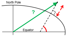
Example 8: “A and azimuth/distance to B”

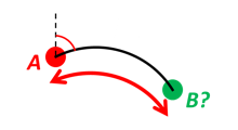
We have an initial position A, direction of travel given as an azimuth (bearing) relative to north (clockwise), and finally the distance to travel along a great circle given as sAB. Use Earth radius 6371e3 m to find the destination point B.

In geodesy this is known as “The first geodetic problem” or “The direct geodetic problem” for a sphere, and we see that this is similar to Example 2, but now the delta is given as an azimuth and a great circle distance. (“The second/inverse geodetic problem” for a sphere is already solved in Examples 1 and 5.)

Solution:

>>> import nvector as nv
>>> from nvector import rad, deg
>>> lat, lon = rad(80), rad(-90)

>>> n_EA_E = nv.lat_lon2n_E(lat, lon)
>>> azimuth = rad(200)
>>> s_AB = 1000.0  # [m]
>>> r_earth = 6371e3  # [m], mean earth radius

Greatcircle solution:

>>> distance_rad = s_AB / r_earth
>>> n_EB_E = nv.n_EA_E_distance_and_azimuth2n_EB_E(n_EA_E, distance_rad, azimuth)
>>> lat_EB, lon_EB = nv.n_E2lat_lon(n_EB_E)
>>> lat, lon = deg(lat_EB), deg(lon_EB)
>>> msg = "Ex8, Destination: lat, lon = {:4.4f} deg, {:4.4f} deg"
>>> msg.format(lat[0], lon[0])
'Ex8, Destination: lat, lon = 79.9915 deg, -90.0177 deg'

Exact solution:

>>> n_EB_E2, azimuthb = nv.geodesic_reckon(n_EA_E, s_AB, azimuth, a=r_earth, f=0)
>>> lat_EB2, lon_EB2 = nv.n_E2lat_lon(n_EB_E2)
>>> lat2, lon2 = deg(lat_EB2), deg(lon_EB2)
>>> msg = "Ex8, Destination: lat, lon = {:4.4f} deg, {:4.4f} deg"
>>> msg.format(lat[0], lon[0])
'Ex8, Destination: lat, lon = 79.9915 deg, -90.0177 deg'

See also

n_EA_E_distance_and_azimuth2n_EB_E, nvector.rotation.E_rotation

nvector.core.great_circle_distance(n_EA_E: List[Any] | Tuple[Any, ...] | ndarray[tuple[Any, ...], dtype[Any]], n_EB_E: List[Any] | Tuple[Any, ...] | ndarray[tuple[Any, ...], dtype[Any]], radius: ArrayLike = 6371009.0) → ndarray[tuple[Any, ...], dtype[floating]]

Returns great circle distance between positions A and B on a sphere

Parameters:

• n_EA_E (List[Any] | Tuple[Any, ...] | npt.NDArray[Any]) – 3 x k array n-vector(s) [no unit] of position A, decomposed in E.

• n_EB_E (List[Any] | Tuple[Any, ...] | npt.NDArray[Any]) – 3 x m array n-vector(s) [no unit] of position B, decomposed in E.

• radius (npt.ArrayLike) – radius of sphere [m]. (default 6371009.0)

Returns:

distance – Array of length max(k, m), great circle distance(s) in meters.

Return type:

npt.NDArray[np.floating]

Notes

The result for spherical Earth is returned. The shape of the output distance is the broadcasted shapes of n_EA_E, n_EB_E and radius. Formula is given by equation (16) in Gade [Gad10] and is well conditioned for all angles. See also: https://en.wikipedia.org/wiki/Great-circle_distance.

Examples

Example 5: “Surface distance”

Find the surface distance sAB (i.e. great circle distance) between two positions A and B. The heights of A and B are ignored, i.e. if they don’t have zero height, we seek the distance between the points that are at the surface of the Earth, directly above/below A and B. The Euclidean distance (chord length) dAB should also be found. Use Earth radius 6371e3 m. Compare the results with exact calculations for the WGS-84 ellipsoid.

Solution for a sphere:

>>> import numpy as np
>>> import nvector as nv
>>> from nvector import rad

>>> n_EA_E = nv.lat_lon2n_E(rad(88), rad(0))
>>> n_EB_E = nv.lat_lon2n_E(rad(89), rad(-170))

>>> r_Earth = 6371e3  # m, mean Earth radius
>>> s_AB = nv.great_circle_distance(n_EA_E, n_EB_E, radius=r_Earth)[0]
>>> d_AB = nv.euclidean_distance(n_EA_E, n_EB_E, radius=r_Earth)[0]

>>> msg = "Ex5: Great circle and Euclidean distance = {}"
>>> msg = msg.format("{:5.2f} km, {:5.2f} km")
>>> msg.format(s_AB / 1000, d_AB / 1000)
'Ex5: Great circle and Euclidean distance = 332.46 km, 332.42 km'

Exact solution for the WGS84 ellipsoid:

>>> p_EA_E = nv.n_EB_E2p_EB_E(n_EA_E, 0)
>>> p_EB_E = nv.n_EB_E2p_EB_E(n_EB_E, 0)
>>> d_12 = np.linalg.norm(p_EA_E-p_EB_E)
>>> s_12, azi1, azi2 = nv.geodesic_distance(n_EA_E, n_EB_E)
>>> msg = "Ellipsoidal and Euclidean distance = {:5.2f} km, {:5.2f} km"
>>> msg.format(s_12 / 1000, d_12 / 1000)
'Ellipsoidal and Euclidean distance = 333.95 km, 333.91 km'

See also

euclidean_distance, geodesic_distance, great_circle_distance_rad

nvector.core.great_circle_distance_rad(n_EA_E: List[Any] | Tuple[Any, ...] | ndarray[tuple[Any, ...], dtype[Any]], n_EB_E: List[Any] | Tuple[Any, ...] | ndarray[tuple[Any, ...], dtype[Any]]) → ndarray[tuple[Any, ...], dtype[floating]]

Returns great circle distance in radians between positions A and B on a sphere

Parameters:

• n_EA_E (List[Any] | Tuple[Any, ...] | npt.NDArray[Any]) – 3 x k array n-vector(s) [no unit] of position A, decomposed in E.

• n_EB_E (List[Any] | Tuple[Any, ...] | npt.NDArray[Any]) – 3 x m array n-vector(s) [no unit] of position B, decomposed in E.

Returns:

distance_rad – Array of length max(k, m), great circle distance(s) in radians

Return type:

npt.NDArray[np.floating]

Notes

The result for spherical Earth is returned. The shape of the output distance_rad is the broadcasted shapes of n_EA_E`and `n_EB_E. Formula is given by equation (16) in Gade [Gad10] and is well conditioned for all angles. See also: https://en.wikipedia.org/wiki/Great-circle_distance.

Examples

Example 5: “Surface distance”

Find the surface distance sAB (i.e. great circle distance) between two positions A and B. The heights of A and B are ignored, i.e. if they don’t have zero height, we seek the distance between the points that are at the surface of the Earth, directly above/below A and B. The Euclidean distance (chord length) dAB should also be found. Use Earth radius 6371e3 m. Compare the results with exact calculations for the WGS-84 ellipsoid.

Solution for a sphere:

>>> import numpy as np
>>> import nvector as nv
>>> from nvector import rad

>>> n_EA_E = nv.lat_lon2n_E(rad(88), rad(0))
>>> n_EB_E = nv.lat_lon2n_E(rad(89), rad(-170))

>>> r_Earth = 6371e3  # m, mean Earth radius
>>> s_AB = nv.great_circle_distance(n_EA_E, n_EB_E, radius=r_Earth)[0]
>>> d_AB = nv.euclidean_distance(n_EA_E, n_EB_E, radius=r_Earth)[0]

>>> msg = "Ex5: Great circle and Euclidean distance = {}"
>>> msg = msg.format("{:5.2f} km, {:5.2f} km")
>>> msg.format(s_AB / 1000, d_AB / 1000)
'Ex5: Great circle and Euclidean distance = 332.46 km, 332.42 km'

Exact solution for the WGS84 ellipsoid:

>>> p_EA_E = nv.n_EB_E2p_EB_E(n_EA_E, 0)
>>> p_EB_E = nv.n_EB_E2p_EB_E(n_EB_E, 0)
>>> d_12 = np.linalg.norm(p_EA_E-p_EB_E)
>>> s_12, azi1, azi2 = nv.geodesic_distance(n_EA_E, n_EB_E)
>>> msg = "Ellipsoidal and Euclidean distance = {:5.2f} km, {:5.2f} km"
>>> msg.format(s_12 / 1000, d_12 / 1000)
'Ellipsoidal and Euclidean distance = 333.95 km, 333.91 km'

See also

great_circle_distance

nvector.core.great_circle_normal(n_EA_E: List[Any] | Tuple[Any, ...] | ndarray[tuple[Any, ...], dtype[Any]], n_EB_E: List[Any] | Tuple[Any, ...] | ndarray[tuple[Any, ...], dtype[Any]]) → ndarray[tuple[Any, ...], dtype[floating]]

Returns the unit normal(s) to the great circle(s)

Parameters:

• n_EA_E (List[Any] | Tuple[Any, ...] | npt.NDArray[Any]) – 3 x k array n-vector [no unit] of position A, decomposed in E.

• n_EB_E (List[Any] | Tuple[Any, ...] | npt.NDArray[Any]) – 3 x m array n-vector [no unit] of position B, decomposed in E.

Returns:

normal – 3 x max(k, m) array of unit normal(s).

Return type:

npt.NDArray[np.floating]

Notes

The shape of the output normal is the broadcasted shapes of n_EA_E and n_EB_E.

nvector.core.interp_nvectors(t_i: ArrayLike, t: ArrayLike, nvectors: List[Any] | Tuple[Any, ...] | ndarray[tuple[Any, ...], dtype[Any]], kind: int | str = 'linear', window_length: int = 0, polyorder: int = 2, mode: str = 'interp', cval: int | float = 0.0) → ndarray[tuple[Any, ...], dtype[floating]]

Returns interpolated values from nvector data.

Parameters:

• t_i (npt.ArrayLike) – Vector of interpolation times of length m.

• t (npt.ArrayLike) – Vector of times of length n.

• nvectors (List[Any] | Tuple[Any, ...] | npt.NDArray[Any]) – 3 x n array of n-vectors [no unit] decomposed in E.

• kind (str or int) – Specifies the kind of interpolation as a string (“linear”, “nearest”, “zero”, “slinear”, “quadratic”, “cubic” where “zero”, “slinear”, “quadratic” and “cubic” refer to a spline interpolation of zeroth, first, second or third order) or as an integer specifying the order of the spline interpolator to use. Default is “linear”.

• window_length (int) – The length of the Savitzky-Golay filter window (i.e., the number of coefficients). Default window_length=0, i.e. no smoothing. Must be positive odd integer or zero.

• polyorder (int) – The order of the polynomial used to fit the samples. polyorder must be less than window_length. Default 2.

• mode (str) – Accepted values are “mirror”, “constant”, “nearest”, “wrap” or “interp”. Determines the type of extension to use for the padded signal to which the filter is applied. When mode is “constant”, the padding value is given by cval. When the “interp” mode is selected (the default), no extension is used. Instead, a degree polyorder polynomial is fit to the last window_length values of the edges, and this polynomial is used to evaluate the last window_length // 2 output values. Default “interp”.

• cval (int or float) – Value to fill past the edges of the input if mode is “constant”. Default is 0.0.

Returns:

Result is 3 x m array of interpolated n-vector(s) [no unit] decomposed in E.

Return type:

npt.NDArray[np.floating]

Notes

The result for spherical Earth is returned.

Examples

>>> import matplotlib.pyplot as plt
>>> import numpy as np
>>> import nvector as nv
>>> lat, lon = nv.rad(np.arange(0, 10)), np.sin(nv.rad(np.linspace(-90, 70, 10)))
>>> t = np.arange(len(lat))
>>> t_i = np.linspace(0, t[-1], 100)
>>> nvectors = nv.lat_lon2n_E(lat, lon)
>>> nvectors_i = nv.interp_nvectors(t_i, t, nvectors, kind="cubic")
>>> lati, loni = nv.deg(*nv.n_E2lat_lon(nvectors_i))
>>> h = plt.plot(nv.deg(lon), nv.deg(lat), "o", loni, lati, "-")
>>> plt.show()
>>> plt.close()

Interpolate noisy data

>>> n = 50
>>> lat = nv.rad(np.linspace(0, 9, n))
>>> lon = np.sin(nv.rad(np.linspace(-90, 70, n))) + 0.05* np.random.randn(n)
>>> t = np.arange(len(lat))
>>> t_i = np.linspace(0, t[-1], 100)
>>> nvectors = nv.lat_lon2n_E(lat, lon)
>>> nvectors_i = nv.interp_nvectors(t_i, t, nvectors, "cubic", 31)
>>> [lati, loni] = nv.n_E2lat_lon(nvectors_i)
>>> h = plt.plot(nv.deg(lon), nv.deg(lat), "o", nv.deg(loni), nv.deg(lati), "-")
>>> plt.show()
>>> plt.close()

nvector.core.interpolate(path: Tuple[List[Any] | Tuple[Any, ...] | ndarray[tuple[Any, ...], dtype[Any]], List[Any] | Tuple[Any, ...] | ndarray[tuple[Any, ...], dtype[Any]]], ti: ArrayLike) → ndarray[tuple[Any, ...], dtype[floating]]

Returns the interpolated point(s) along the path

Parameters:

• path (tuple[List[Any] | Tuple[Any, ...] | npt.NDArray[Any], List[Any] | Tuple[Any, ...] | npt.NDArray[Any]]) – 2-tuple of n-vectors defining the start position A and end position B of the path.

• ti (npt.ArrayLike) – Interpolation time(s) assuming position A and B is at t0=0 and t1=1, respectively. (len(ti) = m).

Returns:

n_EB_E_ti – 3 x m array of interpolated n-vector point(s) along path.

Return type:

npt.NDArray[np.floating]

Notes

The result for spherical Earth is returned.

nvector.core.intersect(path_a: Tuple[List[Any] | Tuple[Any, ...] | ndarray[tuple[Any, ...], dtype[Any]], List[Any] | Tuple[Any, ...] | ndarray[tuple[Any, ...], dtype[Any]]], path_b: Tuple[List[Any] | Tuple[Any, ...] | ndarray[tuple[Any, ...], dtype[Any]], List[Any] | Tuple[Any, ...] | ndarray[tuple[Any, ...], dtype[Any]]]) → ndarray[tuple[Any, ...], dtype[floating]]

Returns the intersection(s) between the great circles of the two paths

Parameters:

• path_a (tuple[List[Any] | Tuple[Any, ...] | npt.NDArray[Any], List[Any] | Tuple[Any, ...] | npt.NDArray[Any]]) – Defining path A with shape 2 x 3 x n

• path_b (tuple[List[Any] | Tuple[Any, ...] | npt.NDArray[Any], List[Any] | Tuple[Any, ...] | npt.NDArray[Any]]) – Defining path B with shape 2 x 3 x m

Returns:

n_EC_E – 3 x max(n, m) array of n-vector(s) [no unit] of position C decomposed in E, which defines the point(s) of intersection between paths.

Return type:

npt.NDArray[np.floating]

Notes

The result for spherical Earth is returned. The shape of the output n_EC_E is the broadcasted shapes of path_a and path_b.

Examples

Example 9: “Intersection of two paths”

Define a path from two given positions (at the surface of a spherical Earth), as the great circle that goes through the two points.

Path A is given by A1 and A2, while path B is given by B1 and B2.

Find the position C where the two great circles intersect.

Solution:

>>> import numpy as np
>>> import nvector as nv
>>> from nvector import rad, deg

>>> n_EA1_E = nv.lat_lon2n_E(rad(10), rad(20))
>>> n_EA2_E = nv.lat_lon2n_E(rad(30), rad(40))
>>> n_EB1_E = nv.lat_lon2n_E(rad(50), rad(60))
>>> n_EB2_E = nv.lat_lon2n_E(rad(70), rad(80))

>>> n_EC_E = nv.unit(np.cross(np.cross(n_EA1_E, n_EA2_E, axis=0),
...                           np.cross(n_EB1_E, n_EB2_E, axis=0),
...                           axis=0))
>>> n_EC_E *= np.sign(np.dot(n_EC_E.T, n_EA1_E))

or alternatively

>>> path_a, path_b = (n_EA1_E, n_EA2_E), (n_EB1_E, n_EB2_E)
>>> n_EC_E = nv.intersect(path_a, path_b)

>>> lat_EC, lon_EC = nv.n_E2lat_lon(n_EC_E)

>>> lat, lon = deg(lat_EC), deg(lon_EC)
>>> msg = "Ex9, Intersection: lat, lon = {:4.4f}, {:4.4f} deg"
>>> msg.format(lat[0], lon[0])
'Ex9, Intersection: lat, lon = 40.3186, 55.9019 deg'

Check that PointC is not between A1 and A2 or B1 and B2:

>>> bool(np.allclose([nv.on_great_circle_path(path_a, n_EC_E),
...                   nv.on_great_circle_path(path_b, n_EC_E)], False))
True

Check that PointC is on the great circle going through path A and path B:

>>> bool(np.allclose([nv.on_great_circle(path_a, n_EC_E),
...                   nv.on_great_circle(path_b, n_EC_E)], True))
True

nvector.core.lat_lon2n_E(latitude: ArrayLike, longitude: ArrayLike, R_Ee: ndarray[tuple[Any, ...], dtype[floating]] | None = None) → ndarray[tuple[Any, ...], dtype[floating]]

Converts latitude and longitude to n-vector.

Parameters:

• latitude (npt.ArrayLike) – Geodetic latitude(s) [rad] (scalar or vector of length n)

• longitude (npt.ArrayLike) – Geodetic longitude(s) [rad] (scalar or vector of length n)

• R_Ee (List[Any] | Tuple[Any, ...] | npt.NDArray[Any]) – Optional 3 x 3 rotation matrix defining the axes of the coordinate frame E. (default E_rotation())

Returns:

n_E – 3 x n array of n-vector(s) [no unit] decomposed in E.

Return type:

npt.NDArray[np.floating]

Examples

>>> import nvector as nv
>>> pi = 3.141592653589793

Scalar call:

>>> bool(nv.allclose(nv.lat_lon2n_E(0, 0), [[1.],
...                                         [0.],
...                                         [0.]]))
True

Vectorized call:

>>> bool(nv.allclose(nv.lat_lon2n_E([0., 0.], [0., pi/2]), [[1., 0.],
...                                                         [0., 1.],
...                                                         [0., 0.]]))
True

Broadcasting call:

>>> bool(nv.allclose(nv.lat_lon2n_E(0., [0, pi/2]), [[1., 0.],
...                                                  [0., 1.],
...                                                  [0., 0.]]))
True

See also

n_E2lat_lon, nvector.rotation.E_rotation

nvector.core.mean_horizontal_position(n_EB_E: ArrayLike) → ndarray[tuple[Any, ...], dtype[floating]]

Returns the n-vector of the horizontal mean position.

Parameters:

n_EB_E (List[Any] | Tuple[Any, ...] | npt.NDArray[Any]) – 3 x n array of n-vectors [no unit] of positions Bi, decomposed in E.

Returns:

p_EM_E – 3 x 1 array of n-vector [no unit] of the mean positions of all Bi, decomposed in E.

Return type:

ndarray

Notes

The result for spherical Earth is returned.

Examples

Example 7: “Mean position”

Three positions A, B, and C are given as n-vectors n_EA_E, n_EB_E, and n_EC_E. Find the mean position, M, given as n_EM_E. Note that the calculation is independent of the depths of the positions.

Solution:

>>> import numpy as np
>>> import nvector as nv
>>> from nvector import rad, deg

>>> n_EA_E = nv.lat_lon2n_E(rad(90), rad(0))
>>> n_EB_E = nv.lat_lon2n_E(rad(60), rad(10))
>>> n_EC_E = nv.lat_lon2n_E(rad(50), rad(-20))

>>> n_EM_E = nv.unit(n_EA_E + n_EB_E + n_EC_E)

or

>>> n_EM_E = nv.mean_horizontal_position(np.hstack((n_EA_E, n_EB_E, n_EC_E)))

>>> lat, lon = nv.n_E2lat_lon(n_EM_E)
>>> lat, lon = deg(lat), deg(lon)
>>> msg = "Ex7: Pos M: lat, lon = {:4.4f}, {:4.4f} deg"
>>> msg.format(lat[0], lon[0])
'Ex7: Pos M: lat, lon = 67.2362, -6.9175 deg'

nvector.core.n_E2lat_lon(n_E: List[Any] | Tuple[Any, ...] | ndarray[tuple[Any, ...], dtype[Any]], R_Ee: List[Any] | Tuple[Any, ...] | ndarray[tuple[Any, ...], dtype[Any]] | None = None) → tuple[ndarray[tuple[Any, ...], dtype[floating]], ndarray[tuple[Any, ...], dtype[floating]]]

Converts n-vector(s) to latitude(s) and longitude(s).

Parameters:

• n_E (List[Any] | Tuple[Any, ...] | npt.NDArray[Any]) – 3 x n array of n-vector(s) [no unit] decomposed in E.

• R_Ee (List[Any] | Tuple[Any, ...] | npt.NDArray[Any]) – 3 x 3 rotation matrix defining the axes of the coordinate frame E, default E_rotation().

Returns:

latitude, longitude – Geodetic latitude(s) and longitude(s) given in [rad]

Return type:

ndarray

See also

lat_lon2n_E, nvector.rotation.E_rotation

nvector.core.n_EA_E_and_n_EB_E2azimuth(n_EA_E: List[Any] | Tuple[Any, ...] | ndarray[tuple[Any, ...], dtype[Any]], n_EB_E: List[Any] | Tuple[Any, ...] | ndarray[tuple[Any, ...], dtype[Any]], a: float = 6378137.0, f: float = 0.0033528106647474805, R_Ee: List[Any] | Tuple[Any, ...] | ndarray[tuple[Any, ...], dtype[Any]] | None = None) → ndarray[tuple[Any, ...], dtype[floating]]

Returns azimuth from A to B, relative to North:

Parameters:

• n_EA_E (List[Any] | Tuple[Any, ...] | npt.NDArray[Any]) – 3 x m array of n-vector(s) [no unit] of position A, decomposed in E.

• n_EB_E (List[Any] | Tuple[Any, ...] | npt.NDArray[Any]) – 3 x n array of n-vector(s) [no unit] of position B, decomposed in E.

• a (float) – Semi-major axis of the Earth ellipsoid given in [m], default WGS-84 ellipsoid.

• f (float) – Flattening [no unit] of the Earth ellipsoid, default WGS-84 ellipsoid. If f==0 then spherical earth with radius a is used instead of WGS-84.

• R_Ee (List[Any] | Tuple[Any, ...] | npt.NDArray[Any]) – Optional 3 x 3 rotation matrix defining the axes of the coordinate frame E, default E_rotation().

Returns:

azimuth – max(m, n) vector of angle(s) [rad] the line(s) makes with a meridian, taken clockwise from north.

Return type:

npt.NDArray[np.floating]

Notes

The shape of the output azimuth is the broadcasted shapes of n_EA_E and n_EB_E.

See also

great_circle_distance_rad, n_EA_E_distance_and_azimuth2n_EB_E, course_over_ground, nvector.rotation.E_rotation

nvector.core.n_EA_E_and_n_EB_E2p_AB_E(n_EA_E: List[Any] | Tuple[Any, ...] | ndarray[tuple[Any, ...], dtype[Any]], n_EB_E: List[Any] | Tuple[Any, ...] | ndarray[tuple[Any, ...], dtype[Any]], z_EA: ArrayLike = 0, z_EB: ArrayLike = 0, a: float = 6378137.0, f: float = 0.0033528106647474805, R_Ee: ndarray[tuple[Any, ...], dtype[floating]] | None = None) → ndarray[tuple[Any, ...], dtype[floating]]

Returns the delta vector from position A to B decomposed in E.

Parameters:

• n_EA_E (List[Any] | Tuple[Any, ...] | npt.NDArray[Any]) – 3 x j array of n-vector(s) [no unit] of position A, decomposed in E.

• n_EB_E (List[Any] | Tuple[Any, ...] | npt.NDArray[Any]) – 3 x k array of n-vector(s) [no unit] of position B, decomposed in E.

• z_EA (npt.ArrayLike) – 1 x m array of depth(s) [m] of system A, relative to the ellipsoid. (z_EA = -height)

• z_EB (npt.ArrayLike) – 1 x n array of depth(s) [m] of system A and B, relative to the ellipsoid. (z_EB = -height)

• a (float) – Semi-major axis of the Earth ellipsoid given in [m], default WGS-84 ellipsoid.

• f (float) – Flattening [no unit] of the Earth ellipsoid. If f==0 then spherical Earth with radius a is used instead of WGS-84, default WGS-84 ellipsoid.

• R_Ee (List[Any] | Tuple[Any, ...] | npt.NDArray[Any]) – Optional 3 x 3 rotation matrix defining the axes of the coordinate frame E, default E_rotation().

Returns:

p_AB_E – 3 x max(j,k,m,n) array of cartesian position vector(s) [m] from A to B, decomposed in E.

Return type:

npt.NDArray[np.floating]

Notes

The n-vectors for positions A (n_EA_E) and B (n_EB_E) are given. The output is the delta vector from A to B decompose in E (p_AB_E). The calculation is exact, taking the ellipsity of the Earth into account. It is also non-singular as both n-vector and p-vector are non-singular (except for the center of the Earth). The default ellipsoid model used is WGS-84, but other ellipsoids/spheres might be specified. The shape of the output p_AB_E is the broadcasted shapes of n_EA_E, n_EB_E, z_EA and z_EB.

Examples

Example 1: “A and B to delta”

Given two positions, A and B as latitudes, longitudes and depths relative to Earth, E.

Find the exact vector between the two positions, given in meters north, east, and down, and find the direction (azimuth) to B, relative to north, as well as elevation and distance.

Assume WGS-84 ellipsoid. The given depths are from the ellipsoid surface. Use position A to define north, east, and down directions. (Due to the curvature of Earth and different directions to the North Pole, the north, east, and down directions will change (relative to Earth) for different places. Position A must be outside the poles for the north and east directions to be defined.)

Solution:

>>> import numpy as np
>>> import nvector as nv
>>> from nvector import rad, deg

>>> lat_EA, lon_EA, z_EA = rad(1), rad(2), 3
>>> lat_EB, lon_EB, z_EB = rad(4), rad(5), 6

Step1: Convert to n-vectors:

>>> n_EA_E = nv.lat_lon2n_E(lat_EA, lon_EA)
>>> n_EB_E = nv.lat_lon2n_E(lat_EB, lon_EB)

Step2: Find p_AB_N (delta decomposed in N). WGS-84 ellipsoid is default:

>>> p_AB_N = nv.n_EA_E_and_n_EB_E2p_AB_N(n_EA_E, n_EB_E, z_EA, z_EB)
>>> x, y, z = p_AB_N.ravel()
>>> "Ex1: delta north, east, down = {0:8.2f}, {1:8.2f}, {2:8.2f}".format(x, y, z)
'Ex1: delta north, east, down = 331730.23, 332997.87, 17404.27'

Step3: Find the direction (azimuth) to B, relative to north as well as elevation and distance:

>>> azimuth = np.arctan2(y, x)
>>> "azimuth = {0:4.2f} deg".format(deg(azimuth))
'azimuth = 45.11 deg'

>>> distance = np.linalg.norm(p_AB_N)
>>> elevation = np.arcsin(z / distance)
>>> "elevation = {0:4.2f} deg".format(deg(elevation))
'elevation = 2.12 deg'

>>> "distance = {0:4.2f} m".format(distance)
'distance = 470356.72 m'

See also

n_EA_E_and_p_AB_E2n_EB_E, n_EA_E_and_n_EB_E2p_AB_N, n_EB_E2p_EB_E, nvector.rotation.E_rotation

nvector.core.n_EA_E_and_n_EB_E2p_AB_N(n_EA_E: List[Any] | Tuple[Any, ...] | ndarray[tuple[Any, ...], dtype[Any]], n_EB_E: List[Any] | Tuple[Any, ...] | ndarray[tuple[Any, ...], dtype[Any]], z_EA: ArrayLike = 0, z_EB: ArrayLike = 0, a: float = 6378137.0, f: float = 0.0033528106647474805, R_Ee: ndarray[tuple[Any, ...], dtype[floating]] | None = None) → ndarray[tuple[Any, ...], dtype[floating]]

Returns the delta vector from position A to B decomposed in N.

Parameters:

• n_EA_E (List[Any] | Tuple[Any, ...] | npt.NDArray[Any]) – 3 x j array of n-vector(s) [no unit] of position A, decomposed in E.

• n_EB_E (List[Any] | Tuple[Any, ...] | npt.NDArray[Any]) – 3 x k array of n-vector(s) [no unit] of position B, decomposed in E.

• z_EA (npt.ArrayLike) – 1 x m array of depth(s) [m] of system A, relative to the ellipsoid. (z_EA = -height)

• z_EB (npt.ArrayLike) – 1 x n array of depth(s) [m] of system A and B, relative to the ellipsoid. (z_EB = -height)

• a (float) – Semi-major axis of the Earth ellipsoid given in [m], default WGS-84 ellipsoid.

• f (float) – Flattening [no unit] of the Earth ellipsoid. If f==0 then spherical Earth with radius a is used in stead of WGS-84, default WGS-84 ellipsoid.

• R_Ee (List[Any] | Tuple[Any, ...] | npt.NDArray[Any]) – Optional 3 x 3 rotation matrix defining the axes of the coordinate frame E, default E_rotation().

Returns:

p_AB_N – 3 x max(j,k,m,n) array of cartesian position vector(s) [m] from A to B, decomposed in N.

Return type:

npt.NDArray[np.floating]

Notes

The n-vectors for positions A (n_EA_E) and B (n_EB_E) are given. The output is the delta vector from A to B decomposed in N (p_AB_N). The calculation is exact, taking the ellipsity of the Earth into account. It is also non-singular as both n-vector and p-vector are non-singular (except for the center of the Earth). The default ellipsoid model used is WGS-84, but other ellipsoids/spheres might be specified. The shape of the output p_AB_N is the broadcasted shapes of n_EA_E, n_EB_E, z_EA and z_EB.

Examples

Example 1: “A and B to delta”

Given two positions, A and B as latitudes, longitudes and depths relative to Earth, E.

Find the exact vector between the two positions, given in meters north, east, and down, and find the direction (azimuth) to B, relative to north, as well as elevation and distance.

Assume WGS-84 ellipsoid. The given depths are from the ellipsoid surface. Use position A to define north, east, and down directions. (Due to the curvature of Earth and different directions to the North Pole, the north, east, and down directions will change (relative to Earth) for different places. Position A must be outside the poles for the north and east directions to be defined.)

Solution:

>>> import numpy as np
>>> import nvector as nv
>>> from nvector import rad, deg

>>> lat_EA, lon_EA, z_EA = rad(1), rad(2), 3
>>> lat_EB, lon_EB, z_EB = rad(4), rad(5), 6

Step1: Convert to n-vectors:

>>> n_EA_E = nv.lat_lon2n_E(lat_EA, lon_EA)
>>> n_EB_E = nv.lat_lon2n_E(lat_EB, lon_EB)

Step2: Find p_AB_N (delta decomposed in N). WGS-84 ellipsoid is default:

>>> p_AB_N = nv.n_EA_E_and_n_EB_E2p_AB_N(n_EA_E, n_EB_E, z_EA, z_EB)
>>> x, y, z = p_AB_N.ravel()
>>> "Ex1: delta north, east, down = {0:8.2f}, {1:8.2f}, {2:8.2f}".format(x, y, z)
'Ex1: delta north, east, down = 331730.23, 332997.87, 17404.27'

Step3: Find the direction (azimuth) to B, relative to north as well as elevation and distance:

>>> azimuth = np.arctan2(y, x)
>>> "azimuth = {0:4.2f} deg".format(deg(azimuth))
'azimuth = 45.11 deg'

>>> distance = np.linalg.norm(p_AB_N)
>>> elevation = np.arcsin(z / distance)
>>> "elevation = {0:4.2f} deg".format(deg(elevation))
'elevation = 2.12 deg'

>>> "distance = {0:4.2f} m".format(distance)
'distance = 470356.72 m'

See also

n_EA_E_and_p_AB_E2n_EB_E, p_EB_E2n_EB_E, n_EB_E2p_EB_E, n_EA_E_and_n_EB_E2p_AB_E, nvector.rotation.E_rotation

nvector.core.n_EA_E_and_p_AB_E2n_EB_E(n_EA_E: List[Any] | Tuple[Any, ...] | ndarray[tuple[Any, ...], dtype[Any]], p_AB_E: List[Any] | Tuple[Any, ...] | ndarray[tuple[Any, ...], dtype[Any]], z_EA: ArrayLike = 0, a: float = 6378137.0, f: float = 0.0033528106647474805, R_Ee: ndarray[tuple[Any, ...], dtype[floating]] | None = None) → tuple[ndarray[tuple[Any, ...], dtype[floating]], ndarray[tuple[Any, ...], dtype[floating]]]

Returns position B from position A and delta vector decomposed in E.

Parameters:

• n_EA_E (List[Any] | Tuple[Any, ...] | npt.NDArray[Any]) – 3 x k array of n-vector(s) [no unit] of position A, decomposed in E.

• p_AB_E (List[Any] | Tuple[Any, ...] | npt.NDArray[Any]) – 3 x m array of cartesian position vector(s) [m] from A to B, decomposed in E.

• z_EA (npt.ArrayLike) – 1 x n array of depth(s) [m] of system A, relative to the ellipsoid. (z_EA = -height).

• a (float) – Semi-major axis of the Earth ellipsoid given in [m], default WGS-84 ellipsoid.

• f (float) – Flattening [no unit] of the Earth ellipsoid. If f==0 then spherical Earth with radius a is used instead of WGS-84, default WGS-84 ellipsoid.

• R_Ee (List[Any] | Tuple[Any, ...] | npt.NDArray[Any]) – Optional 3 x 3 rotation matrix defining the axes of the coordinate frame E, default E_rotation().

Returns:

• n_EB_E (npt.NDArray[np.floating]) – 3 x max(k,m,n) array of n-vector(s) [no unit] of position B, decomposed in E.

• z_EB (npt.NDArray[np.floating]) – 1 x max(k,m,n) array of depth(s) [m] of system B, relative to the ellipsoid. (z_EB = -height).

Notes

The n-vector for position A (n_EA_E) and the delta vector from position A to position B decomposed in E (p_AB_E) are given. The output is the n-vector of position B (n_EB_E) and depth of B (z_EB). The calculation is exact, taking the ellipsity of the Earth into account. It is also non-singular as both n-vector and p-vector are non-singular (except for the center of the Earth). The default ellipsoid model used is WGS-84, but other ellipsoids/spheres might be specified. The shape of the output n_EB_E and z_EB is the broadcasted shapes of n_EA_E, p_AB_E and z_EA.

Examples

Example 2: “B and delta to C”

A radar or sonar attached to a vehicle B (Body coordinate frame) measures the distance and direction to an object C. We assume that the distance and two angles (typically bearing and elevation relative to B) are already combined to the vector p_BC_B (i.e. the vector from B to C, decomposed in B). The position of B is given as n_EB_E and z_EB, and the orientation (attitude) of B is given as R_NB (this rotation matrix can be found from roll/pitch/yaw by using zyx2R).

Find the exact position of object C as n-vector and depth ( n_EC_E and z_EC ), assuming Earth ellipsoid with semi-major axis a and flattening f. For WGS-72, use a = 6 378 135 m and f = 1/298.26.

Solution:

>>> import numpy as np
>>> import nvector as nv
>>> from nvector import rad, deg

A custom reference ellipsoid is given (replacing WGS-84):

>>> wgs72 = dict(a=6378135, f=1.0/298.26)

Step 1 Position and orientation of B is 400m above E:

>>> n_EB_E = nv.unit([[1], [2], [3]])  # unit to get unit length of vector
>>> z_EB = -400
>>> yaw, pitch, roll = rad(10), rad(20), rad(30)
>>> R_NB = nv.zyx2R(yaw, pitch, roll)

Step 2: Delta BC decomposed in B

>>> p_BC_B = np.r_[3000, 2000, 100].reshape((-1, 1))

Step 3: Find R_EN:

>>> R_EN = nv.n_E2R_EN(n_EB_E)

Step 4: Find R_EB, from R_EN and R_NB:

>>> R_EB = np.dot(R_EN, R_NB)  # Note: closest frames cancel

Step 5: Decompose the delta BC vector in E:

>>> p_BC_E = np.dot(R_EB, p_BC_B)

Step 6: Find the position of C, using position n_EB_E and delta vector p_BC_E:

>>> n_EC_E, z_EC = nv.n_EA_E_and_p_AB_E2n_EB_E(n_EB_E, p_BC_E, z_EB, **wgs72)

Step 7: Convert position C to latitude and longitude to make it more convenient to see for humans:

>>> lat_EC, lon_EC = nv.n_E2lat_lon(n_EC_E)
>>> lat, lon, z = deg(lat_EC), deg(lon_EC), z_EC
>>> msg = "Ex2: PosC: lat, lon = {:4.4f}, {:4.4f} deg,  height = {:4.2f} m"
>>> msg.format(lat[0], lon[0], -z[0])
'Ex2: PosC: lat, lon = 53.3264, 63.4681 deg,  height = 406.01 m'

See also

n_EA_E_and_n_EB_E2p_AB_E, p_EB_E2n_EB_E, n_EB_E2p_EB_E, nvector.rotation.E_rotation

nvector.core.n_EA_E_and_p_AB_N2n_EB_E(n_EA_E: List[Any] | Tuple[Any, ...] | ndarray[tuple[Any, ...], dtype[Any]], p_AB_N: List[Any] | Tuple[Any, ...] | ndarray[tuple[Any, ...], dtype[Any]], z_EA: ArrayLike = 0, a: float = 6378137.0, f: float = 0.0033528106647474805, R_Ee: ndarray[tuple[Any, ...], dtype[floating]] | None = None) → tuple[ndarray[tuple[Any, ...], dtype[floating]], ndarray[tuple[Any, ...], dtype[floating]]]

Returns position B from position A and delta vector decomposed in N.

Parameters:

• n_EA_E (List[Any] | Tuple[Any, ...] | npt.NDArray[Any]) – 3 x k array of n-vector(s) [no unit] of position A, decomposed in E.

• p_AB_N (List[Any] | Tuple[Any, ...] | npt.NDArray[Any]) – 3 x m array of cartesian position vector(s) [m] from A to B, decomposed in N.

• z_EA (npt.ArrayLike) – 1 x n array Depth(s) [m] of system A, relative to the ellipsoid. (z_EA = -height)

• a (float) – Semi-major axis of the Earth ellipsoid given in [m], default WGS-84 ellipsoid.

• f (float) – Flattening [no unit] of the Earth ellipsoid. If f==0 then spherical Earth with radius a is used instead of WGS-84, default WGS-84 ellipsoid.

• R_Ee (List[Any] | Tuple[Any, ...] | npt.NDArray[Any]) – Optional 3 x 3 rotation matrix defining the axes of the coordinate frame E, default E_rotation().

Returns:

• n_EB_E (npt.NDArray[np.floating]) – 3 x max(k,m,n) array of n-vector(s) [no unit] of position B, decomposed in E.

• z_EB (npt.NDArray[np.floating]) – 1 x max(k,m,n) array of depth(s) [m] of system B, relative to the ellipsoid. (z_EB = -height)

Notes

The n-vector for position A (n_EA_E) and the delta vector from position A to position B decomposed in N (p_AB_N) are given. The output is the n-vector of position B (n_EB_E) and depth of B (z_EB). The calculation is exact, taking the ellipsity of the Earth into account. It is also non-singular as both n-vector and p-vector are non-singular (except for the center of the Earth). The default ellipsoid model used is WGS-84, but other ellipsoids/spheres might be specified. The shape of the output n_EB_E and z_EB is the broadcasted shapes of n_EA_E, p_AB_N and z_EA.

Examples

Example 2: “B and delta to C”

A radar or sonar attached to a vehicle B (Body coordinate frame) measures the distance and direction to an object C. We assume that the distance and two angles (typically bearing and elevation relative to B) are already combined to the vector p_BC_B (i.e. the vector from B to C, decomposed in B). The position of B is given as n_EB_E and z_EB, and the orientation (attitude) of B is given as R_NB (this rotation matrix can be found from roll/pitch/yaw by using zyx2R).

Find the exact position of object C as n-vector and depth ( n_EC_E and z_EC ), assuming Earth ellipsoid with semi-major axis a and flattening f. For WGS-72, use a = 6 378 135 m and f = 1/298.26.

Solution:

>>> import numpy as np
>>> import nvector as nv
>>> from nvector import rad, deg

A custom reference ellipsoid is given (replacing WGS-84):

>>> wgs72 = dict(a=6378135, f=1.0/298.26)

Step 1 Position and orientation of B is 400m above E:

>>> n_EB_E = nv.unit([[1], [2], [3]])  # unit to get unit length of vector
>>> z_EB = -400
>>> yaw, pitch, roll = rad(10), rad(20), rad(30)
>>> R_NB = nv.zyx2R(yaw, pitch, roll)

Step 2: Delta BC decomposed in B

>>> p_BC_B = np.r_[3000, 2000, 100].reshape((-1, 1))

Step 3: Find R_EN:

>>> R_EN = nv.n_E2R_EN(n_EB_E)

Step 4: Find R_EB, from R_EN and R_NB:

>>> R_EB = np.dot(R_EN, R_NB)  # Note: closest frames cancel

Step 5: Decompose the delta BC vector in E:

>>> p_BC_E = np.dot(R_EB, p_BC_B)

Step 6: Find the position of C, using position n_EB_E and delta vector p_BC_E:

>>> n_EC_E, z_EC = nv.n_EA_E_and_p_AB_E2n_EB_E(n_EB_E, p_BC_E, z_EB, **wgs72)

Step 7: Convert position C to latitude and longitude to make it more convenient to see for humans:

>>> lat_EC, lon_EC = nv.n_E2lat_lon(n_EC_E)
>>> lat, lon, z = deg(lat_EC), deg(lon_EC), z_EC
>>> msg = "Ex2: PosC: lat, lon = {:4.4f}, {:4.4f} deg,  height = {:4.2f} m"
>>> msg.format(lat[0], lon[0], -z[0])
'Ex2: PosC: lat, lon = 53.3264, 63.4681 deg,  height = 406.01 m'

See also

n_EA_E_and_n_EB_E2p_AB_N, n_EA_E_and_p_AB_E2n_EB_E, n_E2R_EN, nvector.rotation.E_rotation

nvector.core.n_EA_E_distance_and_azimuth2n_EB_E(n_EA_E: List[Any] | Tuple[Any, ...] | ndarray[tuple[Any, ...], dtype[Any]], distance_rad: ArrayLike, azimuth: ArrayLike, R_Ee: ndarray[tuple[Any, ...], dtype[floating]] | None = None) → ndarray[tuple[Any, ...], dtype[floating]]

Returns position B from azimuth and distance from position A

Parameters:

• n_EA_E (List[Any] | Tuple[Any, ...] | npt.NDArray[Any]) – 3 x k array n-vector(s) [no unit] of position A, decomposed in E.

• distance_rad (npt.ArrayLike) – m array of great circle distance(s) [rad] from position A to B

• azimuth (npt.ArrayLike) – n array of angle(s) [rad] the line(s) makes with a meridian, taken clockwise from north.

• R_Ee (List[Any] | Tuple[Any, ...] | npt.NDArray[Any]) – Optional 3 x 3 array rotation matrix defining the axes of the coordinate frame E, default E_rotation().

Returns:

n_EB_E – n-vector(s) [no unit] of position B decomposed in E.

Return type:

3 x max(k,m,n) npt.NDArray[np.floating]

Notes

The result for spherical Earth is returned. The shape of the output n_EB_E is the broadcasted shapes of n_EA_E, distance_rad and azimuth.

Examples

Example 8: “A and azimuth/distance to B”

We have an initial position A, direction of travel given as an azimuth (bearing) relative to north (clockwise), and finally the distance to travel along a great circle given as sAB. Use Earth radius 6371e3 m to find the destination point B.

In geodesy this is known as “The first geodetic problem” or “The direct geodetic problem” for a sphere, and we see that this is similar to Example 2, but now the delta is given as an azimuth and a great circle distance. (“The second/inverse geodetic problem” for a sphere is already solved in Examples 1 and 5.)

Solution:

>>> import nvector as nv
>>> from nvector import rad, deg
>>> lat, lon = rad(80), rad(-90)

>>> n_EA_E = nv.lat_lon2n_E(lat, lon)
>>> azimuth = rad(200)
>>> s_AB = 1000.0  # [m]
>>> r_earth = 6371e3  # [m], mean earth radius

Greatcircle solution:

>>> distance_rad = s_AB / r_earth
>>> n_EB_E = nv.n_EA_E_distance_and_azimuth2n_EB_E(n_EA_E, distance_rad, azimuth)
>>> lat_EB, lon_EB = nv.n_E2lat_lon(n_EB_E)
>>> lat, lon = deg(lat_EB), deg(lon_EB)
>>> msg = "Ex8, Destination: lat, lon = {:4.4f} deg, {:4.4f} deg"
>>> msg.format(lat[0], lon[0])
'Ex8, Destination: lat, lon = 79.9915 deg, -90.0177 deg'

Exact solution:

>>> n_EB_E2, azimuthb = nv.geodesic_reckon(n_EA_E, s_AB, azimuth, a=r_earth, f=0)
>>> lat_EB2, lon_EB2 = nv.n_E2lat_lon(n_EB_E2)
>>> lat2, lon2 = deg(lat_EB2), deg(lon_EB2)
>>> msg = "Ex8, Destination: lat, lon = {:4.4f} deg, {:4.4f} deg"
>>> msg.format(lat[0], lon[0])
'Ex8, Destination: lat, lon = 79.9915 deg, -90.0177 deg'

See also

n_EA_E_and_n_EB_E2azimuth, great_circle_distance_rad, geodesic_reckon, nvector.rotation.E_rotation

nvector.core.n_EB_E2p_EB_E(n_EB_E: List[Any] | Tuple[Any, ...] | ndarray[tuple[Any, ...], dtype[Any]], depth: ArrayLike = 0, a: float = 6378137.0, f: float = 0.0033528106647474805, R_Ee: ndarray[tuple[Any, ...], dtype[floating]] | None = None) → ndarray[tuple[Any, ...], dtype[floating]]

Converts n-vector to Cartesian position vector in meters.

Parameters:

• n_EB_E (List[Any] | Tuple[Any, ...] | npt.NDArray[Any]) – 3 x m array of n-vector(s) [no unit] of position B, decomposed in E.

• depth (npt.ArrayLike) – Scalar or 1 x n array of depth(s) [m] of system B, relative to the ellipsoid (depth = -height).

• a (float) – Semi-major axis of the Earth ellipsoid given in [m], default WGS-84 ellipsoid.

• f (float.) – Flattening [no unit] of the Earth ellipsoid. If f==0 then spherical Earth with radius a is used instead

• R_Ee (List[Any] | Tuple[Any, ...] | npt.NDArray[Any] (default E_rotation())) – Optional 3 x 3 rotation matrix defining the axes of the coordinate frame E.

Returns:

p_EB_E – 3 x max(m,n) array of cartesian position vector(s) [m] from E to B, decomposed in E.

Return type:

npt.NDArray[np.floating]

Notes

The position of B (typically body) relative to E (typically Earth) is given into this function as n-vector, n_EB_E. The function converts to cartesian position vector (“ECEF-vector”), p_EB_E, in meters. The calculation is exact, taking the ellipsity of the Earth into account. It is also non-singular as both n-vector and p-vector are non-singular (except for the center of the Earth). The default ellipsoid model used is WGS-84, but other ellipsoids/spheres might be specified. The shape of the output p_EB_E is the broadcasted shapes of n_EB_E and depth.

Examples

Example 4: “Geodetic latitude to ECEF-vector”

Geodetic latitude, longitude and height are given for position B as latEB, lonEB and hEB, find the ECEF-vector for this position, p_EB_E.

Solution:

>>> import nvector as nv
>>> from nvector import rad
>>> wgs84 = dict(a=6378137.0, f=1.0/298.257223563)
>>> lat_EB, lon_EB = rad(1), rad(2)
>>> h_EB = 3
>>> n_EB_E = nv.lat_lon2n_E(lat_EB, lon_EB)
>>> p_EB_E = nv.n_EB_E2p_EB_E(n_EB_E, -h_EB, **wgs84)

>>> "Ex4: p_EB_E = {} m".format(p_EB_E.ravel().tolist())
'Ex4: p_EB_E = [6373290.277218279, 222560.20067473652, 110568.82718178593] m'

See also

p_EB_E2n_EB_E, n_EA_E_and_p_AB_E2n_EB_E, n_EA_E_and_n_EB_E2p_AB_E, nvector.rotation.E_rotation

nvector.core.on_great_circle(path: Tuple[List[Any] | Tuple[Any, ...] | ndarray[tuple[Any, ...], dtype[Any]], List[Any] | Tuple[Any, ...] | ndarray[tuple[Any, ...], dtype[Any]]], n_EB_E: List[Any] | Tuple[Any, ...] | ndarray[tuple[Any, ...], dtype[Any]], radius: ArrayLike = 6371009.0, atol: float = 1e-08) → ndarray[tuple[Any, ...], dtype[bool]]

Returns True if position B is on great circle through path A.

Parameters:

• path (tuple[List[Any] | Tuple[Any, ...] | npt.NDArray[Any], List[Any] | Tuple[Any, ...] | npt.NDArray[Any]]) – 2-tuple of n-vectors of shapes 3 x k and 3 x m, respectively, defining path A, decomposed in E.

• n_EB_E (List[Any] | Tuple[Any, ...] | npt.NDArray[Any]) – 3 x n array n-vector(s) of position B to check to.

• radius (npt.ArrayLike) – Radius of sphere, default 6371009.0. (len(radius)=o)

• atol (float) – The absolute tolerance parameter (See notes).

Returns:

max(k, m, n, o) bool array. An element is True if position B is on great circle through path A.

Return type:

npt.NDArray[np.bool_]

Notes

The default value of atol is not zero, and is used to determine what small values should be considered close to zero. The default value is appropriate for expected values of order unity. However, atol should be carefully selected for the use case at hand. Typically, the value should be set to the accepted error tolerance. For GPS data the error ranges from 0.01 m to 15 m. The shape of the output on is the broadcasted size of n_EB_E, path and radius.

Examples

Example 10: “Cross track distance”

Path A is given by the two positions A1 and A2 (similar to the previous example).

Find the cross track distance sxt between the path A (i.e. the great circle through A1 and A2) and the position B (i.e. the shortest distance at the surface, between the great circle and B).

Also find the Euclidean distance dxt between B and the plane defined by the great circle. Use Earth radius 6371e3.

Finally, find the intersection point on the great circle and determine if it is between position A1 and A2.

Solution:

>>> import numpy as np
>>> import nvector as nv
>>> from nvector import rad, deg
>>> n_EA1_E = nv.lat_lon2n_E(rad(0), rad(0))
>>> n_EA2_E = nv.lat_lon2n_E(rad(10), rad(0))
>>> n_EB_E = nv.lat_lon2n_E(rad(1), rad(0.1))
>>> path = (n_EA1_E, n_EA2_E)
>>> radius = 6371e3  # mean earth radius [m]
>>> s_xt = nv.cross_track_distance(path, n_EB_E, radius=radius)
>>> d_xt = nv.cross_track_distance(path, n_EB_E, method="euclidean",
...                                radius=radius)

>>> val_txt = "{:4.2f} km, {:4.2f} km".format(s_xt[0]/1000, d_xt[0]/1000)
>>> "Ex10: Cross track distance: s_xt, d_xt = {0}".format(val_txt)
'Ex10: Cross track distance: s_xt, d_xt = 11.12 km, 11.12 km'

>>> n_EC_E = nv.closest_point_on_great_circle(path, n_EB_E)
>>> bool(np.allclose(nv.on_great_circle_path(path, n_EC_E, radius), True))
True

Alternative solution 2:

>>> s_xt2 = nv.great_circle_distance(n_EB_E, n_EC_E, radius)
>>> d_xt2 = nv.euclidean_distance(n_EB_E, n_EC_E, radius)
>>> bool(np.allclose(s_xt, s_xt2)), bool(np.allclose(d_xt, d_xt2))
(True, True)

Alternative solution 3:

>>> c_E = nv.great_circle_normal(n_EA1_E, n_EA2_E)
>>> sin_theta = -np.dot(c_E.T, n_EB_E).ravel()
>>> s_xt3 = np.arcsin(sin_theta) * radius
>>> d_xt3 = sin_theta * radius
>>> bool(np.allclose(s_xt, s_xt3)), bool(np.allclose(d_xt, d_xt3))
(True, True)

See also

cross_track_distance

nvector.core.on_great_circle_path(path: Tuple[List[Any] | Tuple[Any, ...] | ndarray[tuple[Any, ...], dtype[Any]], List[Any] | Tuple[Any, ...] | ndarray[tuple[Any, ...], dtype[Any]]], n_EB_E: List[Any] | Tuple[Any, ...] | ndarray[tuple[Any, ...], dtype[Any]], radius: ArrayLike = 6371009.0, atol: float = 1e-08) → ndarray[tuple[Any, ...], dtype[bool]]

Returns True if position B is on great circle and between endpoints of path A.

Parameters:

• path (tuple[List[Any] | Tuple[Any, ...] | npt.NDArray[Any], List[Any] | Tuple[Any, ...] | npt.NDArray[Any]]) – 2-tuple of n-vectors of shapes 3 x k and 3 x m, respectively, defining path A, decomposed in E.

• n_EB_E (List[Any] | Tuple[Any, ...] | npt.NDArray[Any]) – 3 x n array n-vector(s) of position B to measure the cross track distance to.

• radius (npt.ArrayLike) – Radius of sphere. (default 6371009.0)

• atol (real scalars) – The absolute tolerance parameter (See notes).

Returns:

max(k, m, n) bool array. True if position B is on great circle and between endpoints of path A.

Return type:

npt.NDArray[np.bool_]

Notes

The default value of atol is not zero, and is used to determine what small values should be considered close to zero. The default value is appropriate for expected values of order unity. However, atol should be carefully selected for the use case at hand. Typically, the value should be set to the accepted error tolerance. For GPS data the error ranges from 0.01 m to 15 m. The shape of the output on is the broadcasted shapes of n_EB_E path and radius.

Examples

Example 10: “Cross track distance”

Path A is given by the two positions A1 and A2 (similar to the previous example).

Find the cross track distance sxt between the path A (i.e. the great circle through A1 and A2) and the position B (i.e. the shortest distance at the surface, between the great circle and B).

Also find the Euclidean distance dxt between B and the plane defined by the great circle. Use Earth radius 6371e3.

Finally, find the intersection point on the great circle and determine if it is between position A1 and A2.

Solution:

>>> import numpy as np
>>> import nvector as nv
>>> from nvector import rad, deg
>>> n_EA1_E = nv.lat_lon2n_E(rad(0), rad(0))
>>> n_EA2_E = nv.lat_lon2n_E(rad(10), rad(0))
>>> n_EB_E = nv.lat_lon2n_E(rad(1), rad(0.1))
>>> path = (n_EA1_E, n_EA2_E)
>>> radius = 6371e3  # mean earth radius [m]
>>> s_xt = nv.cross_track_distance(path, n_EB_E, radius=radius)
>>> d_xt = nv.cross_track_distance(path, n_EB_E, method="euclidean",
...                                radius=radius)

>>> val_txt = "{:4.2f} km, {:4.2f} km".format(s_xt[0]/1000, d_xt[0]/1000)
>>> "Ex10: Cross track distance: s_xt, d_xt = {0}".format(val_txt)
'Ex10: Cross track distance: s_xt, d_xt = 11.12 km, 11.12 km'

>>> n_EC_E = nv.closest_point_on_great_circle(path, n_EB_E)
>>> bool(np.allclose(nv.on_great_circle_path(path, n_EC_E, radius), True))
True

Alternative solution 2:

>>> s_xt2 = nv.great_circle_distance(n_EB_E, n_EC_E, radius)
>>> d_xt2 = nv.euclidean_distance(n_EB_E, n_EC_E, radius)
>>> bool(np.allclose(s_xt, s_xt2)), bool(np.allclose(d_xt, d_xt2))
(True, True)

Alternative solution 3:

>>> c_E = nv.great_circle_normal(n_EA1_E, n_EA2_E)
>>> sin_theta = -np.dot(c_E.T, n_EB_E).ravel()
>>> s_xt3 = np.arcsin(sin_theta) * radius
>>> d_xt3 = sin_theta * radius
>>> bool(np.allclose(s_xt, s_xt3)), bool(np.allclose(d_xt, d_xt3))
(True, True)

See also

cross_track_distance, on_great_circle

nvector.core.p_EB_E2n_EB_E(p_EB_E: List[Any] | Tuple[Any, ...] | ndarray[tuple[Any, ...], dtype[Any]], a: float = 6378137.0, f: float = 0.0033528106647474805, R_Ee: ndarray[tuple[Any, ...], dtype[floating]] | None = None) → tuple[ndarray[tuple[Any, ...], dtype[floating]], ndarray[tuple[Any, ...], dtype[floating]]]

Converts Cartesian position vector in meters to n-vector.

Parameters:

• p_EB_E (List[Any] | Tuple[Any, ...] | npt.NDArray[Any]) – 3 x n array of cartesian position vector(s) [m] from E to B, decomposed in E.

• a (float) – Semi-major axis of the Earth ellipsoid given in [m], default WGS-84 ellipsoid.

• f (float) – Flattening [no unit] of the Earth ellipsoid. If f==0 then spherical Earth with radius a is used instead of WGS-84, default WGS-84 ellipsoid.

• R_Ee (List[Any] | Tuple[Any, ...] | npt.NDArray[Any]) – Optional 3 x 3 rotation matrix defining the axes of the coordinate frame E, default E_rotation().

Returns:

• n_EB_E (npt.NDArray[np.floating]) – 3 x n array of n-vector(s) [no unit] of position B, decomposed in E.

• depth (npt.NDArray[np.floating]) – 1 x n array of depth(s) [m] of system B, relative to the ellipsoid (depth = -height).

Notes

The position of B (typically body) relative to E (typically Earth) is given into this function as cartesian position vector p_EB_E, in meters. (“ECEF-vector”). The function converts to n-vector, n_EB_E and its depth. The calculation is exact, taking the ellipsity of the Earth into account. It is also non-singular as both n-vector and p-vector are non-singular (except for the center of the Earth). The default ellipsoid model used is WGS-84, but other ellipsoids/spheres might be specified.

Examples

Example 3: “ECEF-vector to geodetic latitude”

Position B is given as an “ECEF-vector” p_EB_E (i.e. a vector from E, the center of the Earth, to B, decomposed in E). Find the geodetic latitude, longitude and height (latEB, lonEB and hEB), assuming WGS-84 ellipsoid.

Solution:

>>> import numpy as np
>>> import nvector as nv
>>> from nvector import deg
>>> wgs84 = dict(a=6378137.0, f=1.0/298.257223563)
>>> p_EB_E = 6371e3 * np.vstack((0.9, -1, 1.1))  # m

Step 1: Find n-vector and depth from the p-vector:

>>> n_EB_E, z_EB = nv.p_EB_E2n_EB_E(p_EB_E, **wgs84)

Step 2: Convert to latitude, longitude and height:

>>> lat_EB, lon_EB = nv.n_E2lat_lon(n_EB_E)
>>> h = -z_EB
>>> lat, lon = deg(lat_EB), deg(lon_EB)

>>> msg = "Ex3: Pos B: lat, lon = {:4.4f}, {:4.4f} deg, height = {:9.3f} m"
>>> msg.format(lat[0], lon[0], h[0])
'Ex3: Pos B: lat, lon = 39.3787, -48.0128 deg, height = 4702059.834 m'

See also

n_EB_E2p_EB_E, n_EA_E_and_p_AB_E2n_EB_E, n_EA_E_and_n_EB_E2p_AB_E, nvector.rotation.E_rotation

5.3. Module related to rotation matrices and angles

5.3.1. Functions in module

E_rotation:

Returns rotation matrix R_Ee defining the axes of the coordinate frame E.

n_E_and_wa2R_EL:

Returns rotation matrix R_EL from n-vector and wander azimuth angle.

n_E2R_EN:

Returns the rotation matrix R_EN from n-vector.

R_EL2n_E:

Returns n-vector from the rotation matrix R_EL.

R_EN2n_E:

Returns n-vector from the rotation matrix R_EN.

R2xyz:

Returns the Euler angles in the xyz-order from a rotation matrix.

R2zyx:

Returns the Euler angles in the zxy-order from a rotation matrix.

xyz2R:

Returns rotation matrix from Euler angles in the xyz-order.

zyx2R:

Returns rotation matrix from Euler angles in the zyx-order.

change_axes_to_E:

Change axes of the nvector(s) from “e” to “E”.

nvector.rotation.E_rotation(axes: str = 'e') → ndarray[tuple[Any, ...], dtype[floating]]

Returns rotation matrix R_Ee defining the axes of the coordinate frame E.

Parameters:

axes (str) – Either “e” or “E” defining the orientation of the axes of the coordinate frame E. If axes is “e” then z-axis points to the North Pole along the Earth’s rotation axis, x-axis points towards the point where latitude = longitude = 0. If axes is “E” then x-axis points to the North Pole along the Earth’s rotation axis, y-axis points towards where longitude +90deg (east) and latitude = 0.

Returns:

R_Ee – 3 x 3 rotation matrix defining the axes of the coordinate frame E as described in Table 2 in the article by Gade [Gad10].

Return type:

ndarray

Notes

R_Ee controls the axes of the coordinate frame E (Earth-Centred, Earth-Fixed, ECEF) used by the other functions in this library. It is very common in many fields to choose axes equal to “e”, which is also the default in this library. Previously the old matlab toolbox the default value was equal to “E”. If you choose axes equal to “E” the yz-plane coincides with the equatorial plane. This choice of axis ensures that at zero latitude and longitude, frame N (North-East-Down) has the same orientation as frame E. If roll/pitch/yaw are zero, also frame B (forward-starboard-down) has this orientation. In this manner, the axes of frame E is chosen to correspond with the axes of frame N and B.

Examples

>>> import numpy as np
>>> import nvector as nv
>>> bool(np.allclose(nv.E_rotation(axes="e"), [[ 0,  0,  1],
...                                            [ 0,  1,  0],
...                                            [-1,  0,  0]]))
True
>>> bool(np.allclose(nv.E_rotation(axes="E"), [[ 1.,  0.,  0.],
...                                            [ 0.,  1.,  0.],
...                                            [ 0.,  0.,  1.]]))
True

nvector.rotation.R2xyz(R_AB: List[Any] | Tuple[Any, ...] | ndarray[tuple[Any, ...], dtype[Any]]) → tuple[floating | ndarray[tuple[Any, ...], dtype[floating]], floating | ndarray[tuple[Any, ...], dtype[floating]], floating | ndarray[tuple[Any, ...], dtype[floating]]]

Returns the Euler angles in the xyz-order from a rotation matrix.

Parameters:

R_AB (List[Any] | Tuple[Any, ...] | npt.NDArray[Any]) – 3 x 3 x n rotation array [no unit] (direction cosine matrix) such that the relation between a vector v decomposed in A and B is given by: v_A = mdot(R_AB, v_B).

Returns:

x, y, z – Angles [rad] of rotation about new axes given as real scalars or vectors of length n.

Return type:

np.floating | npt.NDArray[np.floating]

Notes

The x, y, z angles are called Euler angles or Tait-Bryan angles and are defined by the following procedure of successive rotations: Given two arbitrary coordinate frames A and B. Consider a temporary frame T that initially coincides with A. In order to make T align with B, we first rotate T an angle x about its x-axis (common axis for both A and T). Secondly, T is rotated an angle y about the NEW y-axis of T. Finally, T is rotated an angle z about its NEWEST z-axis. The final orientation of T now coincides with the orientation of B.

The signs of the angles are given by the directions of the axes and the right hand rule.

See also: https://en.wikipedia.org/wiki/Aircraft_principal_axes https://en.wikipedia.org/wiki/Euler_angles https://en.wikipedia.org/wiki/Axes_conventions

See also

xyz2R, R2zyx, xyz2R

nvector.rotation.R2zyx(R_AB: List[Any] | Tuple[Any, ...] | ndarray[tuple[Any, ...], dtype[Any]]) → tuple[floating | ndarray[tuple[Any, ...], dtype[floating]], floating | ndarray[tuple[Any, ...], dtype[floating]], floating | ndarray[tuple[Any, ...], dtype[floating]]]

Returns the Euler angles in the zxy-order from a rotation matrix.

Parameters:

R_AB (List[Any] | Tuple[Any, ...] | npt.NDArray[Any]) – 3 x 3 x n rotation matrix [no unit] (direction cosine matrix) such that the relation between a vector v decomposed in A and B is given by: v_A = mdot(R_AB, v_B).

Returns:

z, y, x – Angles [rad] of rotation about new axes given as real scalars or vectors of length n.

Return type:

np.floating | npt.NDArray[np.floating]

Notes

The z, x, y angles are called Euler angles or Tait-Bryan angles and are defined by the following procedure of successive rotations: Given two arbitrary coordinate frames A and B. Consider a temporary frame T that initially coincides with A. In order to make T align with B, we first rotate T an angle z about its z-axis (common axis for both A and T). Secondly, T is rotated an angle y about the NEW y-axis of T. Finally, T is rotated an angle x about its NEWEST x-axis. The final orientation of T now coincides with the orientation of B.

The signs of the angles are given by the directions of the axes and the right hand rule.

Note that if A is a north-east-down frame and B is a body frame, we have that z=yaw, y=pitch and x=roll.

See also: https://en.wikipedia.org/wiki/Aircraft_principal_axes https://en.wikipedia.org/wiki/Euler_angles https://en.wikipedia.org/wiki/Axes_conventions

See also

zyx2R, xyz2R, R2xyz

nvector.rotation.R_EL2n_E(R_EL: List[Any] | Tuple[Any, ...] | ndarray[tuple[Any, ...], dtype[Any]]) → ndarray[tuple[Any, ...], dtype[floating]]

Returns n-vector from the rotation matrix R_EL.

Parameters:

R_EL (List[Any] | Tuple[Any, ...] | npt.NDArray[Any]) – 3 x 3 x n rotation matrix (direction cosine matrix) [no unit].

Returns:

n_E – 3 x n array of n-vector(s) [no unit] decomposed in E.

Return type:

ndarray

Notes

n-vector is found from the rotation matrix (direction cosine matrix) R_EL.

See also

R_EN2n_E, n_E_and_wa2R_EL, n_E2R_EN

nvector.rotation.R_EN2n_E(R_EN: List[Any] | Tuple[Any, ...] | ndarray[tuple[Any, ...], dtype[Any]]) → ndarray[tuple[Any, ...], dtype[floating]]

Returns n-vector from the rotation matrix R_EN.

Parameters:

R_EN (List[Any] | Tuple[Any, ...] | npt.NDArray[Any]) – 3 x 3 x n rotation matrix (direction cosine matrix) [no unit].

Returns:

n_E – 3 x n array of n-vector [no unit] decomposed in E.

Return type:

ndarray

Notes

n-vector is found from the rotation matrix (direction cosine matrix) R_EN.

See also

n_E2R_EN, R_EL2n_E, n_E_and_wa2R_EL

nvector.rotation.change_axes_to_E(n_E: List[Any] | Tuple[Any, ...] | ndarray[tuple[Any, ...], dtype[Any]], R_Ee: List[Any] | Tuple[Any, ...] | ndarray[tuple[Any, ...], dtype[Any]] | None = None) → ndarray[tuple[Any, ...], dtype[floating]]

Change axes of the nvector(s) from “e” to “E”.

Parameters:

• n_E (List[Any] | Tuple[Any, ...] | npt.NDArray[Any]) – 3 x n array of n-vector(s) [no unit] decomposed in E.

• R_Ee (List[Any] | Tuple[Any, ...] | npt.NDArray[Any]) – 3 x 3 rotation matrix defining the axes of the coordinate frame E, default E_rotation().

Returns:

n_e – 3 x n array of n-vector(s) [no unit] decomposed in e.

Return type:

ndarray

Notes

The function make sure to rotate the coordinates so that axes is “E”: then x-axis points to the North Pole along the Earth’s rotation axis, and yz-plane coincides with the equatorial plane, i.e., y-axis points towards longitude +90deg (east) and latitude = 0.

See also

E_rotation

nvector.rotation.n_E2R_EN(n_E: List[Any] | Tuple[Any, ...] | ndarray[tuple[Any, ...], dtype[Any]], R_Ee: List[Any] | Tuple[Any, ...] | ndarray[tuple[Any, ...], dtype[Any]] | None = None) → ndarray[tuple[Any, ...], dtype[floating]]

Returns the rotation matrix R_EN from n-vector.

Parameters:

• n_E (List[Any] | Tuple[Any, ...] | npt.NDArray[Any]) – 3 x n array of n-vector(s) [no unit] decomposed in E

• R_Ee (List[Any] | Tuple[Any, ...] | npt.NDArray[Any]) – 3 x 3 rotation matrix defining the axes of the coordinate frame E, default E_rotation().

Returns:

R_EN – The resulting 3 x 3 x n rotation matrix [no unit] (direction cosine matrix).

Return type:

ndarray

See also

R_EN2n_E, n_E_and_wa2R_EL, R_EL2n_E, E_rotation

nvector.rotation.n_E_and_wa2R_EL(n_E: List[Any] | Tuple[Any, ...] | ndarray[tuple[Any, ...], dtype[Any]], wander_azimuth: ArrayLike, R_Ee: ndarray[tuple[Any, ...], dtype[floating]] | None = None) → ndarray[tuple[Any, ...], dtype[floating]]

Returns rotation matrix R_EL from n-vector and wander azimuth angle.

Parameters:

• n_E (List[Any] | Tuple[Any, ...] | npt.NDArray[Any]) – 3 x n array of n-vector(s) [no unit] decomposed in E.

• wander_azimuth (npt.ArrayLike) – Angle(s) [rad] between L’s x-axis and north, positive about L’s z-axis given as a real scalar or array of length n.

• R_Ee (List[Any] | Tuple[Any, ...] | npt.NDArray[Any]) – 3 x 3 rotation matrix defining the axes of the coordinate frame E, default E_rotation().

Returns:

R_EL – The resulting 3 x 3 x n rotation matrix. [no unit]

Return type:

ndarray

Notes

Calculates the rotation matrix (direction cosine matrix) R_EL using n-vector (n_E) and the wander azimuth angle. When wander_azimuth`=0, we have that N=L. (See Table 2 in Gade :cite:`Gade2010Nonsingular for details)

See also

R_EL2n_E, R_EN2n_E, n_E2R_EN, nvector.rotation.E_rotation

nvector.rotation.xyz2R(x: ArrayLike, y: ArrayLike, z: ArrayLike) → ndarray[tuple[Any, ...], dtype[floating]]

Returns rotation matrix from Euler angles in the xyz-order.

Parameters:

• x (npt.ArrayLike) – Angles [rad] of rotation about new axes given as real scalars or array of lengths n.

• y (npt.ArrayLike) – Angles [rad] of rotation about new axes given as real scalars or array of lengths n.

• z (npt.ArrayLike) – Angles [rad] of rotation about new axes given as real scalars or array of lengths n.

Returns:

R_AB – 3 x 3 x n rotation matrix [no unit] (direction cosine matrix) such that the relation between a vector v decomposed in A and B is given by: v_A = mdot(R_AB, v_B).

Return type:

ndarray

Notes

The rotation matrix R_AB is created based on 3 angles x,y,z about new axes (intrinsic) in the order x-y-z. The angles are called Euler angles or Tait-Bryan angles and are defined by the following procedure of successive rotations: Given two arbitrary coordinate frames A and B. Consider a temporary frame T that initially coincides with A. In order to make T align with B, we first rotate T an angle x about its x-axis (common axis for both A and T). Secondly, T is rotated an angle y about the NEW y-axis of T. Finally, T is rotated an angle z about its NEWEST z-axis. The final orientation of T now coincides with the orientation of B.

The signs of the angles are given by the directions of the axes and the right hand rule.

See also: https://en.wikipedia.org/wiki/Aircraft_principal_axes https://en.wikipedia.org/wiki/Euler_angles https://en.wikipedia.org/wiki/Axes_conventions

See also

R2xyz, zyx2R, R2zyx

nvector.rotation.zyx2R(z: ArrayLike, y: ArrayLike, x: ArrayLike) → ndarray[tuple[Any, ...], dtype[floating]]

Returns rotation matrix from Euler angles in the zyx-order.

Parameters:

• z (npt.ArrayLike) – Angles [rad] of rotation about new axes given as real scalars or arrays of lenths n.

• y (npt.ArrayLike) – Angles [rad] of rotation about new axes given as real scalars or arrays of lenths n.

• x (npt.ArrayLike) – Angles [rad] of rotation about new axes given as real scalars or arrays of lenths n.

Returns:

R_AB – 3 x 3 x n rotation matrix [no unit] (direction cosine matrix) such that the relation between a vector v decomposed in A and B is given by: v_A = mdot(R_AB, v_B).

Return type:

ndarray

Notes

The rotation matrix R_AB is created based on 3 angles z,y,x about new axes (intrinsic) in the order z-y-x. The angles are called Euler angles or Tait-Bryan angles and are defined by the following procedure of successive rotations: Given two arbitrary coordinate frames A and B. Consider a temporary frame T that initially coincides with A. In order to make T align with B, we first rotate T an angle z about its z-axis (common axis for both A and T). Secondly, T is rotated an angle y about the NEW y-axis of T. Finally, T is rotated an angle x about its NEWEST x-axis. The final orientation of T now coincides with the orientation of B.

The signs of the angles are given by the directions of the axes and the right hand rule.

Note that if A is a north-east-down frame and B is a body frame, we have that z=yaw, y=pitch and x=roll.

See also: https://en.wikipedia.org/wiki/Aircraft_principal_axes https://en.wikipedia.org/wiki/Euler_angles https://en.wikipedia.org/wiki/Axes_conventions

Examples

Suppose the yaw angle between coordinate system A and B is 45 degrees. Convert position p1_b = (1, 0, 0) in B to a point in A. Convert position p2_a =(0, 1, 0) in A to a point in B.

Solution:

>>> import numpy as np
>>> import nvector as nv
>>> x, y, z = nv.rad(0, 0, 45)
>>> R_AB = nv.zyx2R(z, y, x)

>>> p1_b = np.atleast_2d((1, 0, 0)).T
>>> p1_a = nv.mdot(R_AB, p1_b)
>>> bool(nv.allclose(p1_a, [[0.7071067811865476], [0.7071067811865476], [0.0]]))
True

>>> p2_a = np.atleast_2d((0, 1, 0)).T
>>> p2_b = nv.mdot(R_AB.T, p2_a)
>>> bool(nv.allclose(p2_b, [[0.7071067811865476], [0.7071067811865476], [0.0]]))
True

See also

R2zyx, xyz2R, R2xyz

5.4. Utility functions

5.4.1. Functions in module

deg:

Converts angle in radians to degrees.

rad:

Converts angle in degrees to radians.

mdot:

Returns multiple matrix multiplications of two arrays.

i.e. dot(a, b)[i,j,k] = sum(a[i,:,k] * b[:,j,k])

nthroot:

Returns the n’th root of x to machine precision

get_ellipsoid:

Returns semi-major axis (a), flattening (f) and name of reference ellipsoid as a named tuple.

unit:

Convert input vector to a vector of unit length.

isclose:

Returns True where the two arrays a and b are element-wise equal within a tolerance.

allclose:

Returns True if two arrays are element-wise equal within a tolerance.

eccentricity2:

Returns the first and second eccentricity squared given the flattening, f.

polar_radius:

Returns the polar radius b given the equatorial radius a and flattening f of the ellipsoid.

third_flattening:

Returns the third flattening, n, given the flattening, f.

array_to_list_dict:

Convert dict arrays to dict of lists.

dm2degrees:

Converts degrees, minutes to decimal degrees

degrees2dm:

Converts decimal degrees to degrees and minutes.

nvector.util.allclose(a: ArrayLike, b: ArrayLike, rtol: float = 1e-07, atol: float = 1e-14, equal_nan: bool = False) → bool

Returns True if two arrays are element-wise equal within a tolerance.

Parameters:

• a (npt.ArrayLike) – First input array or number to compare.

• b (npt.ArrayLike) – Second input array or number to compare.

• rtol (float) – The relative tolerance parameter (see Notes).

• atol (float) – The absolute tolerance parameter (see Notes).

• equal_nan (bool) – Whether to compare NaN’s as equal. If True, NaN’s in a will be considered equal to NaN’s in b in the output array.

Returns:

Returns np.True_ if the two arrays are equal within the given tolerance; np.False_ otherwise.

Return type:

bool

See also

isclose, all, any, equal

Notes

For finite values, allclose uses the following equation to test whether two floating point values are equivalent:

absolute(a - b) <= maximimum(atol, rtol * maximum(absolute(a), absolute(b)))

NaNs are treated as equal if they are in the same place and if equal_nan=True. Infs are treated as equal if they are in the same place and of the same sign in both arrays.

The comparison of a and b uses standard broadcasting, which means that a and b need not have the same shape in order for allclose(a, b) to evaluate to True.

For NumPy version 2, the representation of its boolean types are np.True_ and np.False_ when returned whereas True and False when they are members of arrays, respectively.

Examples

>>> from nvector.util import allclose
>>> allclose([1e10, 1e-7], [1.00001e10, 1e-8])
False
>>> allclose([1e10, 1e-8], [1.00001e10, 1e-9])
False
>>> allclose([1e10, 1e-8], [1.0001e10, 1e-9])
False
>>> allclose([1.0, np.nan], [1.0, np.nan])
False
>>> allclose([1.0, np.nan], [1.0, np.nan], equal_nan=True)
True

nvector.util.array_to_list_dict(data: Any | ArrayLike | Dict[Any, Any]) → Any | Dict[Any, Any] | List[Any]

Convert dict arrays to dict of lists.

Parameters:

data (Any, ndarray, list, tuple or dict) – A collection of data.

Return type:

dict or list

Notes

If the input is not iterable, then the data is returned untouched.

Examples

>>> import numpy as np
>>> data1 = dict(a=np.zeros((3,)), b=(1,2,3), c=[], d=1, e="test",
...              f=np.nan, g=[1], h=[np.nan], i=None)
>>> e1 = array_to_list_dict(data1)
>>> e1 == {"a": [0.0, 0.0, 0.0],  "b": [1, 2, 3], "c": [],"d": 1,
...        "e": "test", "f": np.nan, "g": [1], "h": [np.nan], "i": None}
True
>>> data2 = [1, 2., None]
>>> e2 = array_to_list_dict(data2)
>>> e2 == [1, 2., None]
True
>>> e3 = array_to_list_dict(np.array([-3., -2., -1.]))
>>> e3 == [-3., -2., -1.]
True
>>> e4 = array_to_list_dict(True)
>>> e4 is True
True

nvector.util.deg(*rad_angles: ArrayLike) → floating | ndarray[tuple[Any, ...], dtype[floating]] | tuple[floating | ndarray[tuple[Any, ...], dtype[floating]], ...]

Converts angle in radians to degrees.

Parameters:

rad_angles (npt.ArrayLike) – Angle in radians.

Returns:

deg_angles – Angle in degrees.

Return type:

np.floating | npt.NDArray[np.floating] | tuple[np.floating | npt.NDArray[np.floating], …]

Examples

>>> import numpy as np
>>> from nvector.util import deg, allclose
>>> deg_number = deg(np.pi/2)
>>> deg_number.size == 1
True
>>> deg_number.item()
90.0
>>> degs_array = deg(np.linspace(0, np.pi, 3))
>>> isinstance(degs_array, np.ndarray)
True
>>> allclose(degs_array, [0., 90., 180.])
True
>>> degs_tuple = deg(np.pi/2, [0, np.pi])
>>> isinstance(degs_tuple, tuple)
True
>>> for value, expected in zip(degs_tuple, (90.0, [  0., 180.])):
...     allclose(value, expected)
True
True

See also

rad

Notes

For NumPy version 2, the representation of its numeric types has changed. The representation of float64 for 90 is np.float64(90.0)

nvector.util.degrees2dm(degrees: ArrayLike) → tuple[integer | ndarray[tuple[Any, ...], dtype[integer]], floating | ndarray[tuple[Any, ...], dtype[floating]]]

Converts decimal degrees to degrees and minutes.

Parameters:

degrees (npt.ArrayLike) – Angles to convert to degrees and minutes.

Returns:

• degs (np.integer | npt.NDArray[np.integer]) – Angles rounded to nearest lower integer.

• minutes (np.floating | npt.NDArray[np.floating]) – Angle in degree minutes.

Examples

>>> from nvector.util import degrees2dm, allclose
>>> allclose(degrees2dm(10.822051), (10, 49.32306))
True
>>> allclose(degrees2dm(10.155385),(10, 9.3231))
True
>>> allclose(degrees2dm(1.155385), (1, 9.3231))
True
>>> allclose(degrees2dm(1.15539), (1, 9.3234))
True
>>> allclose(degrees2dm(-1.15539), (-1, -9.3234))
True
>>> allclose(degrees2dm(-0.15539), (0, -9.3234))
True

See also

dm2degrees

nvector.util.dm2degrees(degrees: ArrayLike, minutes: ArrayLike) → floating | ndarray[tuple[Any, ...], dtype[floating]]

Converts degrees, minutes to decimal degrees

Parameters:

• degrees (npt.ArrayLike) – Angles in integer degrees.

• minutes (npt.ArrayLike) – Angle in degree minutes.

Returns:

deg – Angles to converted to decimal degrees.

Return type:

np.floating | npt.NDArray[np.floating]

Examples

>>> from nvector.util import dm2degrees, allclose
>>> allclose(dm2degrees(10, 49.3231), 10.822051)
True
>>> allclose(dm2degrees(10, 9.3231), 10.155385)
True
>>> allclose(dm2degrees(1, 9.3231), 1.155385)
True
>>> allclose(dm2degrees(-1, -9.3231), -1.155385)
True

>>> allclose(dm2degrees(0, -9.3234), -0.15539)
True

See also

degrees2dm

nvector.util.eccentricity2(f: float | ndarray[tuple[Any, ...], dtype[floating]]) → tuple[float | ndarray[tuple[Any, ...], dtype[floating]], float | ndarray[tuple[Any, ...], dtype[floating]]]

Returns the first and second eccentricity squared given the flattening, f.

Parameters:

f (float or ndarray) – Flattening parameter.

Returns:

e2, e2m – First and second eccentricities, respectively.

Return type:

float or ndarray

Notes

The (first) eccentricity squared is defined as e2 = f*(2-f). The second eccentricity squared is defined as e2m = e2 / (1 - e2).

nvector.util.get_ellipsoid(name: int | str) → Ellipsoid

Returns semi-major axis (a), flattening (f) and name of reference ellipsoid as a named tuple.

Parameters:

name (int or str) –

Name (case insensitive) of ellipsoid or integral enumeration. Valid options are:

1. Airy 1858

2. Airy Modified

3. Australian National

4. Bessel 1841

5. Clarke 1880

6. Everest 1830

7. Everest Modified

8. Fisher 1960

9. Fisher 1968

10. Hough 1956

11. Hayford / International ellipsoid 1924 / European Datum 1950 / ED50

12. Krassovsky 1938

13. NWL-9D / WGS 66

14. South American 1969

15. Soviet Geod. System 1985

16. WGS 72

17. Clarke 1866 / NAD27

18. GRS80 / WGS84 / NAD83

19. ETRS89 / EUREF89

20. NGO1948

Returns:

An instance of an nvector.util.Ellipsoid named tuple.

Return type:

Ellipsoid

Notes

See also: https://en.wikipedia.org/wiki/Geodetic_datum https://en.wikipedia.org/wiki/Reference_ellipsoid

Examples

>>> from nvector.util import get_ellipsoid
>>> get_ellipsoid(name="wgs84")
Ellipsoid(a=6378137.0, f=0.0033528106647474805, name='GRS80 / WGS84 / NAD83')
>>> get_ellipsoid(name="GRS80")
Ellipsoid(a=6378137.0, f=0.0033528106647474805, name='GRS80 / WGS84 / NAD83')
>>> get_ellipsoid(name="NAD83")
Ellipsoid(a=6378137.0, f=0.0033528106647474805, name='GRS80 / WGS84 / NAD83')
>>> get_ellipsoid(name=18)
Ellipsoid(a=6378137.0, f=0.0033528106647474805, name='GRS80 / WGS84 / NAD83')

>>> wgs72 = get_ellipsoid(name="WGS 72")
>>> wgs72.a == 6378135.0
True
>>> wgs72.f == 0.003352779454167505
True
>>> wgs72.name
'WGS 72'
>>> wgs72 == (6378135.0, 0.003352779454167505, 'WGS 72')
True

nvector.util.isclose(a: ArrayLike, b: ArrayLike, rtol: float = 1e-09, atol: float = 0.0, equal_nan: bool = False) → ndarray[tuple[Any, ...], dtype[bool]]

Returns True where the two arrays a and b are element-wise equal within a tolerance.

Parameters:

• a (npt.ArrayLike) – First input array or number to compare.

• b (npt.ArrayLike) – Second input array or number to compare.

• rtol (float) – The relative tolerance parameter (see Notes).

• atol (float) – The absolute tolerance parameter (see Notes).

• equal_nan (bool) – Whether to compare NaN’s as equal. If True, NaN’s in a will be considered equal to NaN’s in b in the output array.

Returns:

Returns a boolean array of where a and b are equal within the given tolerance. If both a and b are scalars, returns a single boolean value.

Return type:

ndarray

See also

allclose

Notes

For finite values, isclose uses the following equation to test whether two floating point values are equivalent:

absolute(a - b) <= maximimum(atol, rtol * maximum(absolute(a), absolute(b)))

Like the built-in math.isclose, the above equation is symmetric in a and b. Furthermore, atol should be carefully selected for the use case at hand. A zero value for atol will result in False if either a or b is zero.

For NumPy version 2, the representation of its boolean types are np.True_ and np.False_ when returned whereas True and False when they are members of arrays, respectively.

Examples

>>> import numpy as np
>>> from nvector.util import isclose
>>> bool(np.all(isclose([1e10,1e-7], [1.00001e10,1e-8]) == [False, False]))
True
>>> bool(np.all(isclose([1e10,1e-8], [1.00001e10,1e-9]) == [False, False]))
True
>>> bool(np.all(isclose([1e10,1e-8], [1.0001e10,1e-9]) == [False, False]))
True
>>> bool(np.all(isclose([1.0, np.nan], [1.0, np.nan]) == [True, False]))
True
>>> bool(np.all(isclose([1.0, np.nan], [1.0, np.nan], equal_nan=True) == [True, True]))
True
>>> bool(np.all(isclose([1e-8, 1e-7], [0.0, 0.0]) == [False, False]))
True
>>> bool(np.all(isclose([1e-100, 1e-7], [0.0, 0.0], atol=0.0) == [False, False]))
True
>>> bool(np.all(isclose([1e-10, 1e-10], [1e-20, 0.0]) == [False, False]))
True
>>> bool(np.all(isclose([1e-10, 1e-10], [1e-20, 0.999999e-10], atol=0.0) == [False, False]))
True

nvector.util.mdot(a: List[Any] | Tuple[Any, ...] | ndarray[tuple[Any, ...], dtype[Any]], b: List[Any] | Tuple[Any, ...] | ndarray[tuple[Any, ...], dtype[Any]]) → ndarray[tuple[Any, ...], dtype[floating]]

Returns multiple matrix multiplications of two arrays. i.e. dot(a, b)[i,j,k] = sum(a[i,:,k] * b[:,j,k])

Parameters:

• a (List[Any] | Tuple[Any, ...] | npt.NDArray[Any]) – First argument.

• b (List[Any] | Tuple[Any, ...] | npt.NDArray[Any]) – Second argument.

Returns:

Matrix multiplication of a and b

Return type:

ndarray

Notes

if a and b have the same shape this is the same as

np.concatenate([np.dot(a[…,i], b[…,i])[:, :, None] for i in range(n)], axis=2)

Examples

3 x 3 x 2 times 3 x 3 x 2 array -> 3 x 3 x 2 array

>>> import numpy as np
>>> from nvector.util import mdot, allclose
>>> a = 1.0 * np.arange(18).reshape(3,3,2)
>>> b = - a
>>> t = np.concatenate(
...     [np.dot(a[...,i], b[...,i])[:, :, None] for i in range(2)],
...     axis=2)
>>> tm = mdot(a, b)
>>> tm.shape
(3, 3, 2)
>>> allclose(t, tm)
True

3 x 3 x 2 times 3 x 1 array -> 3 x 1 x 2 array

>>> t1 = np.concatenate([np.dot(a[...,i], b[:,0,0][:,None])[:,:,None]
...                    for i in range(2)], axis=2)

>>> tm1 = mdot(a, b[:,0,0].reshape(-1,1))
>>> tm1.shape
(3, 1, 2)
>>> allclose(t1, tm1)
True

3 x 3 times 3 x 3 array -> 3 x 3 array

>>> tt0 = mdot(a[..., 0], b[..., 0])
>>> tt0.shape
(3, 3)
>>> allclose(t[..., 0], tt0)
True

3 x 3 times 3 x 1 array -> 3 x 1 array

>>> tt0 = mdot(a[..., 0], b[:, :1, 0])
>>> tt0.shape
(3, 1)
>>> allclose(t[:, :1, 0], tt0)
True

3 x 3 times 3 x 1 x 2 array -> 3 x 1 x 2 array

>>> tt0 = mdot(a[..., 0], b[:, :2, 0][:, None])
>>> tt0.shape
(3, 1, 2)
>>> allclose(t[:, :2, 0][:,None], tt0)
True

See also

numpy.einsum

nvector.util.nthroot(x: ArrayLike, n: int) → floating | ndarray[tuple[Any, ...], dtype[floating]]

Returns the n’th root of x to machine precision

Parameters:

• x (npt.ArrayLike) – Value.

• n (int) – Integral root.

Return type:

np.floating | npt.NDArray[np.floating]

Examples

>>> from nvector.util import allclose, nthroot
>>> allclose(nthroot(27.0, 3), 3.0)
True
>>> allclose(nthroot([27.0, 64.0, 125.0], 3), [3, 4, 5])
True

nvector.util.polar_radius(a: float | ndarray[tuple[Any, ...], dtype[floating]], f: float | ndarray[tuple[Any, ...], dtype[floating]]) → float | ndarray[tuple[Any, ...], dtype[floating]]

Returns the polar radius b given the equatorial radius a and flattening f of the ellipsoid.

Parameters:

• a (float or ndarray) – Equatorial radius.

• f (float or ndarray) – Flattening parameter.

Returns:

b – Polar radius

Return type:

float or ndarray

Notes

The semi minor half axis (polar radius) is defined as where is the semi major half axis (equatorial radius) and is the flattening of the ellipsoid.

nvector.util.rad(*deg_angles: ArrayLike) → floating | ndarray[tuple[Any, ...], dtype[floating]] | tuple[floating | ndarray[tuple[Any, ...], dtype[floating]], ...]

Converts angle in degrees to radians.

Parameters:

deg_angles (npt.ArrayLike) – Angle in degrees.

Returns:

rad_angles – Angle in radians.

Return type:

np.floating | npt.NDArray[np.floating] | tuple[np.floating | npt.NDArray[np.floating], …]

Examples

>>> import numpy as np
>>> from nvector.util import deg, rad, allclose
>>> allclose(deg(rad(90)), 90)
True
>>> degs_tuple = deg(*rad(90, [0, 180]))
>>> isinstance(degs_tuple, tuple)
True
>>> for value, expected in zip(degs_tuple, (90.0, [  0., 180.])):
...     allclose(value, expected)
True
True

See also

deg

Notes

For NumPy version 2, the representation of its numeric types has changed. The representation of float64 for 90 is np.float64(90.0)

nvector.util.third_flattening(f: float | ndarray[tuple[Any, ...], dtype[floating]]) → float | ndarray[tuple[Any, ...], dtype[floating]]

Returns the third flattening, n, given the flattening, f.

Parameters:

f (float or ndarray) – Flattening parameter.

Returns:

n – Third flattening .

Return type:

float or ndarray

Notes

The third flattening is defined as .

nvector.util.unit(vector: List[Any] | Tuple[Any, ...] | ndarray[tuple[Any, ...], dtype[Any]], norm_zero_vector: int | float = 1, norm_zero_axis: int = 0) → ndarray[tuple[Any, ...], dtype[floating]]

Convert input vector to a vector of unit length.

Parameters:

• vector (List[Any] | Tuple[Any, ...] | npt.NDArray[Any]) – 3 x m array (m column vectors).

• norm_zero_vector (int | float) – Defines the fill value used for zero length vectors. Either 1 or NaN.

• norm_zero_axis (int) – Defines the direction that zero length vectors will point after the normalization is done.

Returns:

3 x m array, normalized unit-vector(s) along axis==0.

Return type:

ndarray

Notes

The column vector(s) that have zero length will be returned as unit vector(s) pointing in the x-direction, i.e, [[1], [0], [0]] if norm_zero_vector is one, otherwise NaN.

Examples

>>> from nvector.util import unit, allclose
>>> allclose(unit([[1, 0],[1, 0],[1, 0]]), [[ 0.57735027, 1],
...                                         [ 0.57735027, 0],
...                                         [ 0.57735027, 0]])
True